
| Introduction |
| Contents |
| Getting Started |
| Download |
| Navigating |
| Tutorials |
| Scripting |
| Advanced |
| About |
HEMI 2
The hyper-envelope modeling interface allows you to create habitat suitability models from points where species have been observed and covariate raster layers. The "Quick Start" section below will get you started with HEMI. Then, move on to the additional web pages at the bottom of this page. There is also help available in each of the HEMI dialog boxes by pressing the "Help" button.
Quick Start
Creating and evaluating accurate habitat suitability models requires some training and some time. The steps below will just get you started with HEMI 2.
- Gather a set of points where a particular species has been observed.
- Gather a set of rasters containing environmental variables that will co-vary with the species required habitat. Examples include temperature, precipitation, land cover, distance to streams, roughness measures.
- Load both data sets into BlueSpray
- Right click on the point layer and select Wizards -> HEMI 2
- The dialog that appears will allow you to add the covariate rasters by selecting then in the popup menu and clicking the plus ("+") button.
- The next window that appears is the main window for HEMI 2 and allows you to dynamically, or automatically create and evaluate habitat suitability models. Click the "Fit" button to have HEMI 2 automatically fit models to your occurrence and covariate data. In a moment, you should see the curves in the "Model" panels fit to your occurrence data in red.
- Clicking "Map" will display a predicted habitat map in the window on the right and will compute overall statistics for the map.
- Right click on the map and you can "send it scene". This will render a full-resolution map into BlueSpray which you can examine and save to a file.
- You've just run your first model but there is much more to explore and do. Below are some of the features to explore:
- Change the covariate layers to new layers that can be used to predict the species range in a new area or under different scenarios such as climate change
- Edit the points on the model manually based on information that is missing from the occurrences
- Evaluate the model with cross-validation and sensitivity testing.
- Produce uncertainty maps showing the confidence for the habitat map.
The Main Dialog
All of the features mentioned above can be accessed by accessing the menu items, clicking on buttons, and right clicking on the panels in the HEMI 2 window. We invite you to explore HEMI 2 at this time and then continue with this help information.
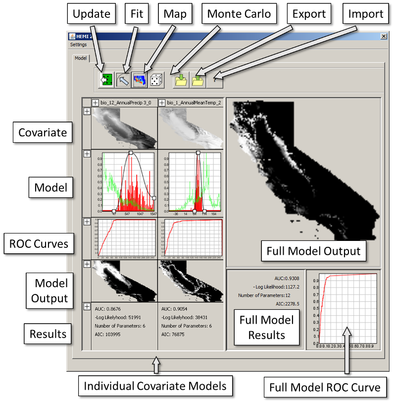
The Window Elements
Below is a short explanation of each of the elements in the HEMI 2 window.
Settings Menu
In the "Settings" menu, you'll find a menu item to change the covariates for the models to perform predictions.
Action Buttons
Update Button
When you first enter the HEMI 2 window, it will automatically update the charts based on the occurrences and covariates you selected. If you change the covariate sin the "Settings" menu, you'll need to press "Update" to see the new data in the charts.
Fit Button
This button will fit the models to the available data.
Map Button
The map button will create a final model by combining all the covariates together.
Monte Carlo Button
This button will open the settings dialog for the Monte Carlo operations which combine validation, sensitivity testing, and uncertainty analysis into a single operation.
Export Button
The export button will save your model to a SchoonerTurtles file (".stx" extension) so you can load it in again later.
Import Button
This button will load a model back into HEMI 2 that was exported.
Individual Covariate Models
The left side of the main panel in HEMI 2 contains columns for each of the covariates. There are controls that initially show plus signs ("+") above each column and to the left of each row. These are controls that allow you to show or hide the rows and columns. In addition, you can right click on the plus sign at the top of any column to set whether to use a covariate in the current model.
Covariate
The first row contains small views of the covariate rasters. These rasters will not change and can be hidden by clicking on the plus sign ("+") on the left.
Model
The second row contains the current models for each covariate. In green is a histogram of the covariate values while red shows the histogram of the occurrences. Both histograms have been scaled so their maximum value is one (i.e. uses the full vertical range of the chart). In black is the model itself. The small boxes are control points that you can drag to change the model. This will update the covariate row but not the overall model. For that, you need to click the map button.
You can right click on the Model to; change the type of the model, fit the model to the occurrences, and export the chart to the clipboard or a file.
ROC Curve
The Receiver Operator Curve (ROC) shows how well the model fits the occurrences given the entire sample area. It is desired to have the area under the curve sum to one which occurs when the curve moves from the bottom-left quickly up to the top-left and then over to the top-right. Changing the points on the model will automatically update the ROC curve.
You can right click on the ROC Curve to export the chart to the clipboard or a file.
Model Output
The model output is a small version of the model if only one covariate was used in the model.
Results
The results panel shows the result statistics for each covariate model. These include:
- AUC: Area Under The Curve computed from the ROC curve above. Values near 1 are considered good models while 0.5 would be random
- -Log Likelihood: A probability measure of how well the model fits the occurrences. A smaller value is desired as this is computed by multiplying all the modeled probabilities of all the occurrences together and then taking the natural log of the result.
- Number of Parameters: The number of estimated (manually or automatically) parameters in the model.
- AIC: Akaike's Information Criterion should be minimized to find the "best" model. AIC is computed using AIC=2*NumParameters-2 Log Likelihood
Note that these values will vary slightly from those in the full model even if you create a model from only a single covariate. This is because we use the histograms in the model to compute the values for the results. This makes it possible for you to dynamically edit the models and immediately see the results. However, the histograms "quantize" the values and thus make the results slightly different from those for the full model which are computed directly from the final model.
Full Model
On the right side of the window, the full model will appear with its statistics.
Full Model Output
This is the final habitat suitability model and you can export it to the scene your occurrences are in in BlueSpray by right clicking on the model.
Full Model Results
These results are the same as those for the covariate models except they are computed based on the entire model. Note that the two sets of results are computed in slightly different ways so the values will vary slightly if even if you use only one covariate in your model.
Full Model ROC Curve
This is a curve based on the final model including all the covariate models you included in the final model.
Additional Help Pages