| Introduction |
| Contents |
| Getting Started |
| Download |
| Navigating |
| Tutorials |
| Scripting |
| Advanced |
| About |
HEMI Models with Synthetic Data
Below is a walk through of using synthetic data to show how HEMI 2 can create models from occurrences. Using synthetic data (data created by a computer program instead of collected outside) is a method to evaluate a modeling package under controlled circumstances. This allows us to show that HEMI 2 can recreate an original habitat niche for a species. Subsequent pages will show how HEMI models uncertainty in the data.
Let's suppose that the images below are both covariates for a plant's habitat preference in a specified environment. The one on the left could be mean annual temperature with the minimum temperature on the left and the maximum on the right. The one on the right could be precipitation with the minimum on the bottom and the maximum on the top.
 |
 |
| Covariate values from 0 (left) to 255 (right) | Covariate with values form 0 (top) to 255 (bottom) |
|---|
Below are shown hypothetical responses of the species to each of the covariates above.
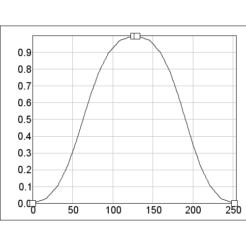
Below are show the response surfaces for each of the curves above when used against each of the covariates. These show that the species prefers the area down the center of the first covariate while the species preferred the middle of the second. At the left and right of the first covariate are areas that are habitat for the species (e.g. too cold or too hot), similarly, the area at the top and bottom of the second covariate are inhospitable (e.g. too wet or too dry).


Combining these together gives the hypothetical habitat for the species. This would also represent the "fundamental habitat" for the species.

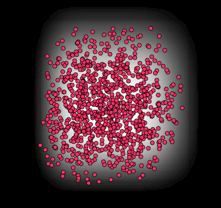
We can then add hypothetical occurrences based on an unbiased sampling method. In other words, the image below shows what might happen if we randomly sampled the area above using a uniform random sample across the area. This also assumes that the plant has fully saturated all of it's available habitat. The image below contains 1000 occurrences, notice how there are more occurrences in the center.
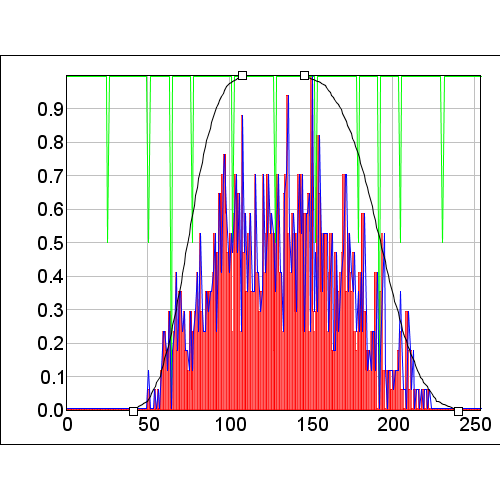
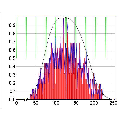
Modeling using these covariates shows a number of important items. In the graphs below, the "LeftToRight" covariate is shown on the left and the "TopToBottom" covariate on the right. The green histogram shows the values from the covariate while the red histogram is the histogram of the covariate values at the occurrences. The blue histogram is the occurrence histogram divided by the covariate histogram to scale the occurrences based on the available habitat. Since the available habitat is effective uniform in this synthetically created data, the two occurrence histograms are identical.
We can see that the sampling of only 1000 points has left us with histograms that have a much higher level of complexity than out original species response. This is a direct result of simply having too few occurrences to cover the environmental niche. This is made worse each time we add a covariate.
The models shown were optimized using the default settings in HEMI 2 which optimize for AIC.
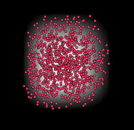
Below is a modeled habitat map using the models above. We can see that the map is very similar to the original habitat map with the habit expanding slightly.