
| Introduction |
| Contents |
| Getting Started |
| Download |
| Navigating |
| Tutorials |
| Scripting |
| Advanced |
| About |
Correcting for Bias
One of the sources of uncertainty in occurrences is bias due either to the current distribution of a species or how the sampling was conducted. Some species, such as invasive species, may not have fully occupied their ecological niche and may be moving across a landscape. Also, much of the data we have available for occurrences for species was not sampled using a random or uniform method but was "opportunistically" collected. This means the data may have a bias. One example is that more data tends to be available near roads because of the ease of access. Because roads only occupy a portion of the landscape, this can lead to a bias or shift in the data that results in a shift in a habitat model. Fortunately, if we know the nature of the bias, this is one of the few areas of uncertainty that we can correct for to some extent.
Let's suppose that we have a road running through the habitat from the previous example. This can create a bias in our data that we will have more occurrences near the road than away from it.
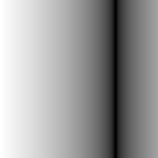
Figure 1. Distance to a road that could cause a bias in our sampling design.
If we set the maximum distance from the road in our sampling region and then set the road as 1 and raise the result to the power of 6, we have a raster that represents the amount of bias that occurred near the road (1.0) vs. at the maximum distance to the road (Figure 2).

Figure 2.
If we multiply the bias times the original habitat and then randomly place occurrences based on our biased habitat/sampling raster, we can see the occurrences have shifted toward the road (Figure 3).
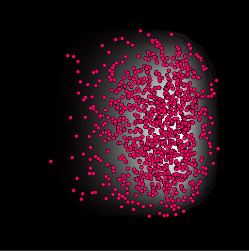
Figure 3. The result of a bias sampling design has shifted the occurrences toward the road.
Now, if we create a model from the occurrences above, we will have a model that is shifted in the environmental space (Figure 4).
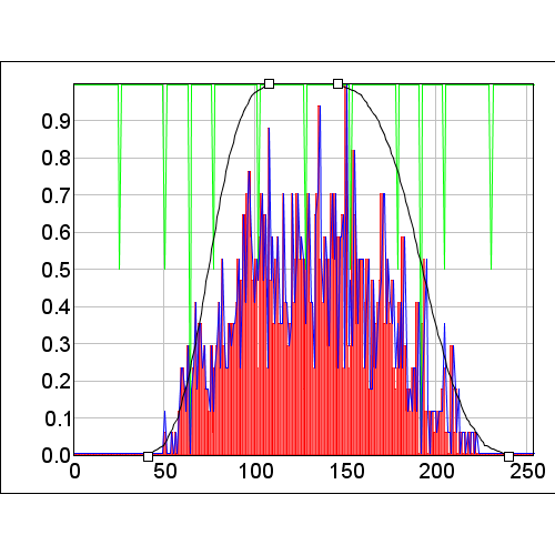
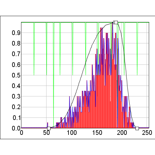
Figure 4. The original model is on the left with the new biased model on the right.
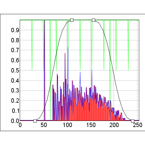
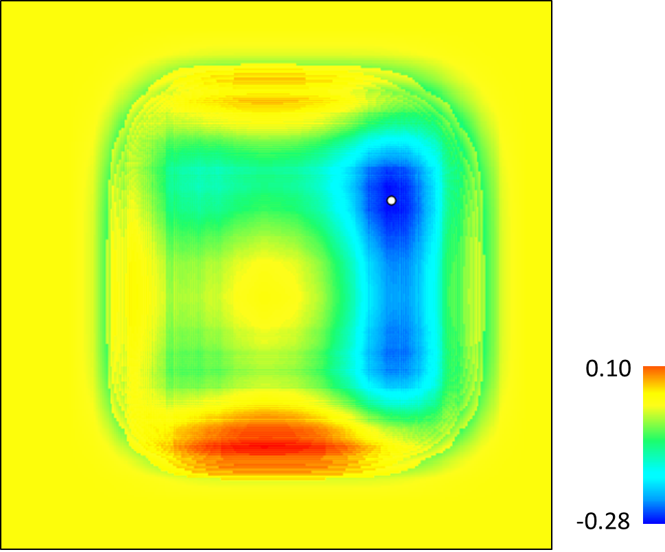
Figure 5. Model with the biased corrected.
While the biased correction raster allowed us to shift the model back to where it should be, notice that the magnitude of the changes on the left of the model are much greater than those on the right. This is because when we corrected for bias, we make the rare occurrences have more value so where there were occurrences we see high values and, since there were fewer points on the left, we see larger gaps in the data.