Lab 1: Introduction to Software and Remote Sensing Applications
Introduction
In this lab exercise we will become acquainted with the computer lab and/or Vlab interface, Google Drive folders and software. The lab will provide an introduction to the image processing software ENVI, including how to open satellite imagery, navigate and perform basic functions in ENVI. This lab will also explore recent developments and applications in remote sensing through a series of new articles.
Learning Outcomes
Learn about and describe some of the recent applications of remote sensing
Establish an understanding of the data storage, using a standardized folder structure and where/how to properly back-up data
How to download and extract compressed files (ZIP/7Z files)
Use ENVI interface to view files, navigate and measure features in imagery
Export images from ENVI and how to insert images into documents to create professional figures
Part 1: Remote Sensing News Articles Summary
Read/listen/watch the below remote sensing focused articles. Summarize and discuss the articles in a one to two page write-up, a minimum of 500s word total. Include the following items in your write-up:
Summarize and briefly discuss each of the following articles.
Discuss which article was most interesting to you and why.
What do these articles tell you about the future of remote sensing?
For most of the lab assignments in this course, we will be utilizing ENVI, an image processing software program. ENVI is industry-standard geospatial image processing and analysis software used by researchers, GIS professionals, and analysts to process and extract meaningful information from various remote sensing datasets.
You will begin by creating a folder structure or "workspace" that will keep your files organized and prevent any confusion as you work with multiple datasets in the future. It is important to have the files you are working stored with on a local drive (C: in our case). Most processes in ENVI and ArcGIS do not work well (or at all!) when data is stored in the cloud (i.e. Google Drive G: Drive), class share network drive (Z: Drive) or on portable USB storage devices.
About the Data
The imagery in this lab exercise include two satellite images of the Arcata, McKinleyville area. The first, recent image, was collected in January 2026 by one of Planet's PlanetScope Dove satellites. The second image shows the same region, but in March 2010. The historic 2010 image was captured by the RapidEye satellite constellation, which is now part of the Planet data collection.
Create a new folder on the local desktop by following the below steps:
Right click the Desktop
Click on New → Folder
Name the folder “GSP216_Lab_01”. Your folder should be located C:\Users\abc123\Desktop (abc123 will be your Humboldt user name). If you are working on your personal computer you may choose to change the directory location but keep the general file structure the same.
In future labs you will want to back up your final work onto a USB drive, or cloud based storage like Google Drive or the ClassShare Network Drive). The hard drives (including the desktop) on the lab computers will be deleted every 24 hours. Be sure to always save and backup your work!
Open up your favorite web browser, log into myHumboldt and navigate to your Humboldt Google Drive. Find the GSP 216 Remote Sensing folder that has been shared with you (under Shared with me) or follow the link to the shared Google Drive folder on the Canvas home page under resources. All of the lab data for this course can be found in the Lab Data folder. In the Lab Data folder locate the file “Lab1Data.zip”, Right Click on this file and select “Download”.
Move the ZIP file from your Downloads folder into your Lab 1 folder on your desktop. You can do this by dragging the file or by right clicking and copying and pasting the downloaded file into the folder.
Right click on the file “Lab1Data.zip” and select “Extract All”. Now the files have been uncompressed and are ready to view.
Go to Start Menu and "ENVI 6.2”. This will open the ENVI software package. Do not open ENVI Classic or ENVI Lidar, they are different programs. We will be using ENVI 6.2 for most of the lab assignments.
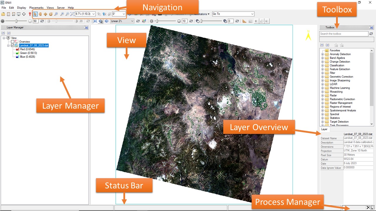
Once ENVI has launched, open the first satellite image by navigating to File → Open and navigate to the desktop and locate the Lab_01 folder. Find and select the file “Arcata01122026.dat” and click Open. You may need to wait a minute for the image to fully load. The below image shows an overview of the ENVI interface for reference.
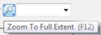
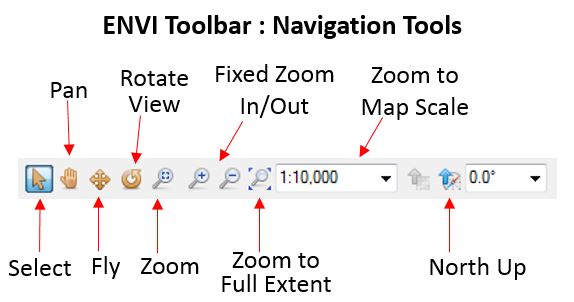
You now should see a recent satellite image of the Arcata area of northern California in your ENVI viewer. This image was acquired by Planet's PlanetScope Dove satellites. Use the navigation tools in the toolbar to explore the image. These tools include pan, fly, zoom. The Zoom to Full Extent Tool zooms out to show the entire extent of the image in the viewer. Watch the video below for an overview of the ENVI navigation tools.
You can use the Brightness controls to darken or brighten the selected image. The valid range is 0 (dark) to 100 (bright), to return to the default value of 50, click the Reset Brightness button. You can also adjust the Sharpness and Transparency of each layer. Experiment with the different controls to see their impact. Note that the brightness/sharpness/transparency adjustments are all temporary and do not change the actual image file.
Image Window Views
In ENVI, there are several tools that help you visualize the extent and geographic location of data. The Overview option shows a thumbnail of the raster and defines the extent currently shown in the view. Another useful tool is the Reference Map Link that opens up a new window with a variety of Esri base maps that correspond to the geographic extent of the raster in the viewer.
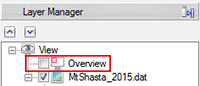
First let's explore the Overview option. To show the Overview, click the Overview check box for the desired View in the Layer Manager window.
The Overview appears in the top-left corner of each Image window view. The Overview Locater, a rectangle within the Overview, defines the extent to show in the view. As you move around the image the locator rectangle moves accordingly. Turn off the Overview by clicking the disable the check box.
Now let’s get an idea of the geographic area and terrain that this image covers. From the menu bar select View → Reference Map Link. This opens up a new window with a base map that shows the geographic extent of the raster in the viewer. Note: this feature is only available on Windows, not on Mac. Click the Switch Basemap drop-down list and select a different type of base map (satellite image, topographic, streets, etc.). After you’re done exploring, you can close the basemap window.
Now we will open a historic image of the same region acquired by Planet's RapidEye satellites. This image from March 2010 shows the same region . Go to File → Open and select the file “Arcata03102010.dat” in your Lab_01 folder and click open.
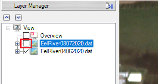
Explore the image by zooming in on difference areas to get an idea of what you can see in the image and how to navigate in ENVI. You can toggle between the two layers by checking/unchecking the boxes by the file names in the layer manager.
Now let's check out Blend, Flicker and Swipe tools that can be used to compare layers. These are found in the main toolbar . First click on the "Blend" icon in the toolbar . This creates an animation that blends or fades between the two selected layers. Click on the "Flicker" icon in the toolbar. This creates an animation that switches between the two layer. Finally click on the "Swipe" icon in the toolbar. This creates an animation that swipes between the two layer. Use these tools to compare the images.
Turn off the "Swipe" animation by clicking on the swipe icon again or right clicking on the "View Swipe" in the Layer Manager and selecting "Remove" or by clicking on the "X" in the upper right hand corner.
Click the "Zoom to full Extent". This button to zooms to the full extent of the data layer. You should now be able see the entire satellite image centered in your viewer. The next steps go over how to take export images for use in reports or presentation.
We will frequently be taking screenshots or exporting imagery in this course. Screenshots are an easy way to include images and figures into reports. Screenshots are also an easy to show someone what you're seeing on your computer screen instead of trying explaining it. Learn More About Taking Screenshots. There are many different options on how to take screenshots or export imagery in ENVI, the below video details some of the many options.
Make sure only the recent image is visible, you can do this by unchecking the older image. We will now learn to use the "Chip to View" option in ENVI to save the current view as an image. This option is very similar to taking a screenshot. Make sure you view is set to the full extent before exporting the image.
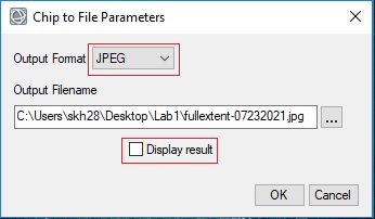
Go to File > Chip View To >File in ENVI. Select "JPEG" as the output file type and uncheck"Display Results."
Save the jpeg in your Lab 1 folder. File names should not include spaces or special characters, I recommend including either the location or description as well as a date in the name.
Check your lab folder to verify that the image has been saved.
Without moving the image or zooming in/out, uncheck the current image in the layer manager and check the historic image to turn it on. You should now see the full extent of the 2010 image in your viewer. Repeat the above step and but this time use the "Chip to View" to export an image showing the full extent image in 2010. You will now have two exported images saved, both showing the full extent of the satellite images (one from 2010 and one from 2026).
Taking Measurements
Now we will learn how to measure linear features and distances using the tools in ENVI. Click the Mensuration button in the Toolbar . The Cursor Value dialog appears, and red cross-hairs are displayed over the center of the view. The cursor icon changes to a + symbol, indicating that it is ready to draw line segments.
Practice using the measuring tool by measuring a length of road or other feature. To measure a distance, click on the image to start measuring and click a second time once you have reached the end of the feature you are measuring. Then right click and select Accept, the line segment becomes a polyline annotation that is added to the Layer Manager. The measurement distance for the polyline is displayed in the Cursor Value window. Click the Units drop-down list in the Cursor Value dialog to change them.
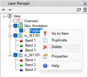
Now we will delete our practice measurement polyline. In the Layer Manager, expand the New Annotation heading by click the + icon, now you will see the Polyline you just created. Right click on the polyline in layer manager and select Delete. This will remove the Polyline and measurements.
Find the mouth of the Mad River (Baduwa't), using the Reference Map link to help you locate it (step 10). Toggle the two image layers on and off or use the Blend, Flicker and Swipe tools to compare layers. Note that the mouth of the river has moved significantly over the past 15 years.
Measure the distance between the mouth of the Mad River between the two time periods. Adjust the Transparency (see step 8) of the layer or turn the layers on and off to accurately measure, or you may also use the use the Blend, Flicker and Swipe tools to help. After measuring the distance, click the Units drop-down list in the Cursor Value dialog, and select US Survey Feet. Note the distance, you will include this information in your lab report. Turn off the annotations in the layer manager by unchecking the box (optional, you may also leave the annotation on if you like the look of it in the final image).
Now we will Chip the View (or export the screenshot) but this time zoomed in the mouth of the Mad River. Use the zoom and navigation tools to focus in on the mouth of the river. Once you are centered on your area of interest use the Chip to View to to export a jpeg of the image.
Now export an image of the same area from the other time period. Without moving the image or zooming in/out, check the other image file in the layer manager, this will toggle on/off imagery. Use the Chip to View to to export a jpeg of the same area of interest from the other time time period. You should have a total of four image, two showing the full extent and two zoomed in on the mouth of the Mad River. Make sure to write down the distance the mouth has moved, as you will include this in now of the captions for the figures.
Open up a new blank document in Microsoft Word (or Google Doc, but you will need to save the file as a Word document or PDF for submission). Use the insert image/picture function in Word to insert your saved images. This will insert your exported image into your document. If necessary, screenshots or image exports should always be cropped appropriately and only include the necessary imagery.
You should have four images in your document: full extent of the two satellite images, and two zoomed in on the mouth of the Mad River.
Include a caption for each your figures (4). Note that captions should always be labeled with the figure number (i.e. Figure 1.) in bold followed by a description of the figure. An example for a different dataset would be: "Figure 1. Sentinel-2 satellite image of Lake Tahoe region acquired in September 2021". Adjust your captions to match your imagery, one of the captions should include the distance the mouth of the river has moved. Captions for figures should be placed below images or figures. You also need to include your name, the date and class (GSP 216) on your document. Save the document in your Lab 1 folder.
Back up your completed work by either transferring your complete files (document and exported images) to Google Drive, the ClassShare Z: Drive or a personal USB drive. There is no need to back-up the original imagery, as it is always available on the class Google Drive or on the ClassShare Z: Drive. You may close ENVI when you are done. Part I and II may be complete as separate documents or you may combine the two parts into one document for submission.
Save and Restore Session in ENVI
Unlike ArcGIS Pro, ENVI is not project based. That means it is typically not necessary to save your project (known as workspace or session in ENVI) before closing ENVI. If you would like to preserve your current work environment, you can do this by Saving an ENVI Session. This does not save the actual data files (similar to saving a map project in ArcGIS) but saves a link to the open data files, layout configuration, and display enhancements (like zoom, stretch, and transparency). You must also back up the original geospatial data as well. The session is saved as a JSON-formatted file (.json) with references to the data location, layers and display settings.
To save your current workspace in ENVI, select File > ENVI Session > Save from the menu bar. Save the .json session file, which saves the locations of the files and settings. To re-open a saved session in ENVI, select File > ENVI Session > Restor and open the JSON file with the saved session. Watch Saving ENVI Session for more information.
Contact Info
Humboldt State University
1 Harpst Street Arcata, CA 95521
skh28@humboldt.edu

 First let's explore the Overview option. To show the Overview, click the Overview check box for the desired View in the Layer Manager window.
The Overview appears in the top-left corner of each Image window view. The Overview Locater, a rectangle within the Overview, defines the extent to show in the view. As you move around the image the locator rectangle moves accordingly. Turn off the Overview by clicking the disable the check box.
First let's explore the Overview option. To show the Overview, click the Overview check box for the desired View in the Layer Manager window.
The Overview appears in the top-left corner of each Image window view. The Overview Locater, a rectangle within the Overview, defines the extent to show in the view. As you move around the image the locator rectangle moves accordingly. Turn off the Overview by clicking the disable the check box.