Working with lidar data in FUSION
Introduction
This lab will introduce you to several ways of visializing point cloud lidar data and calculate a few topography and forest metrics. You will familiarize yourself with FUSION, a lidar viewing and analysis software tool developed by the Silviculture and Forest Models Team, Research Branch of the US Forest Service. The software can be downloaded and used for free. For more details follow this link : About FUSION. We will use data from the State of Washington in the WGS 1984 UTM Zone 10N coordinate system.
Workspace set up
This lab will go easier if you have a well-organized folder structure to select raw data from and store intermediate and final results.
- On the Desktop create a folder called lidarlab.
- Download the labdata from here: Lidar lab data and save it in your lidarlab folder.
- Extract the data : Right click on the zip file and choose 7-Zip then Extract Here. Delete the zipped file whem done.
- Now you should have a structure like the one shown below:
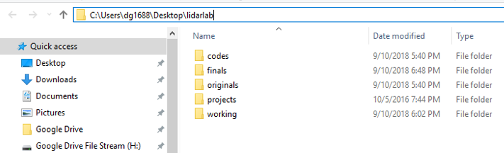
It will save you a lot of time if you have your workspace exactly like this because the codes we will use for forest metrics calculations are based on this workspace organization, thus all you will have to do is replace “dg1688” with your log in ID and you will be good to go. However, if you have your workspace set otherwise, you need to edit a lot of the code’s components, which may end up confusing or frustrating.
Part 1: Basics of FUSION
- Start Fusion – Click on the Windows Icon and type “FUSION”.
- Click on the FUSION Icon. If you cannot find FUSION this way, navigate to the C:\FUSION folder and then double click fusion.exe
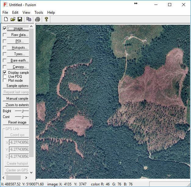
We will use an orthophotograph to visualize the data
- Click the Image button located on Fusion toolbar (left panel). Navigate to your “originals” folder and select the orthophoto (demo_4800k_UTM.jpg) and Click, Open.
The image will automatically display in the Fusion viewer. If you want to zoom-in to any part of the image, Right Click on the location you want to zoom to. Zoom-out by Clicking the Zoom to extents button on the left panel.
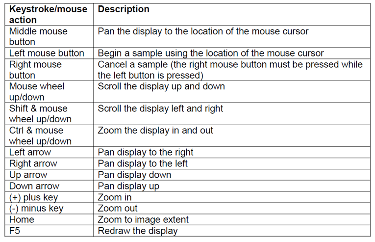
You can zoom in and out, or pan the image using the mouse or keyboard functions described in Appendix 1
Now add the raw point cloud lidar data
- Click the Raw Data button on the Fusion toolbar to display the Open dialog box.
- Navigate to your “originals” folder and Select the sample dataset (demo_4800k_UTM.lda) and Click, Open. This will open the Data Files dialog.
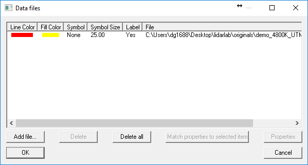
The Data Files dialog allows you to change the display Symbology of the lidar data in the Fusion window but, it is strongly recommended that you accept the defaults (especially the Symbol set to None) for now:
- Click OK
- Save your Fusion project to your “projects” folder by Clicking the Save icon or File|Save As.
- Name the project lidarlab.dvz
View the lidar data in the Lidar Data Viewer (LDV)
To create a sample and view the corresponding Lidar data in 3D:
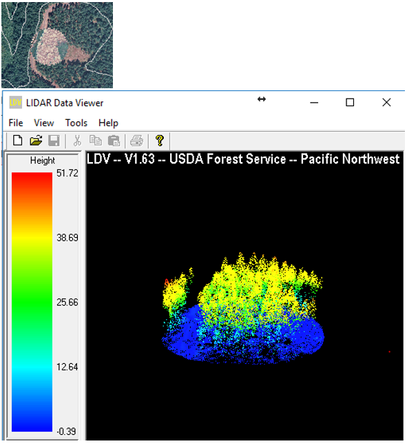
- Position the cursor over an area of interest in the orthophoto, Left Click and drag a small box (called a stroked box) over the area and release the left mouse button—this is your sample. Note: a small sample works better (faster) than a large sample.
The sample box will be highlighted in the Fusion viewer and LDV, Fusion’s 3D viewer, will automatically appear and load the Lidar data within your sample boundary, as in the figure below.
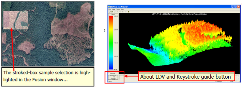
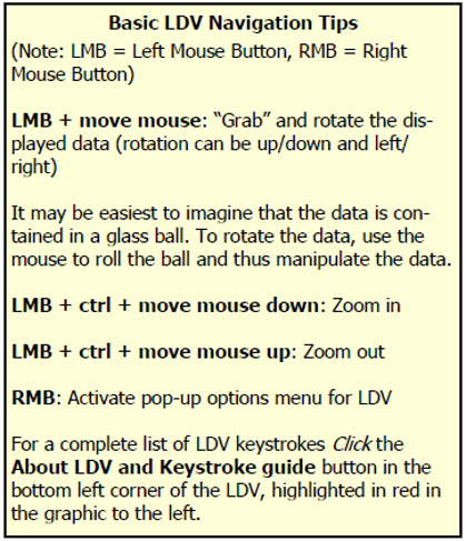
- 10. Use the Basic LDV Navigation Tips (sidebar) until you are comfortable with your ability to control the data cloud.
Add a Bare Earth (Ground) Model
- Close the LDV and return to FUSION (it will still be running & your last sampled area will be displayed).
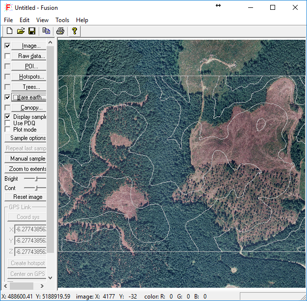
- Click the Bare earth button (located on the Fusion toolbar).
- Navigate to your “originals” folder and select the sample terrain model (demo_4800K_UTM.dtm) and Click, Open.
- Within the Surface model options window, accept the defaults.
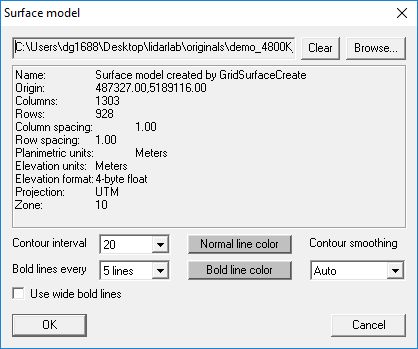
- Click, OK. The terrain model will be displayed in the Fusion viewer as a contour map over the orthophoto.
- Click the “Repeat last sample” button (located on the Fusion toolbar). This will display the same lidar data cloud as before—but in a moment we will also view the bare earth surface.
- Right Click within the LDV viewer to access the “Right Click Menu”.
- Click on Surfaces (or use the Alt-U keyboard option). The bare earth surface will automatically display with your lidar data cloud.
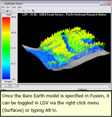
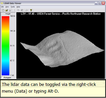
- Access the right-click menu again and Click on Data to toggle the data off (or type Alt-D).
- This will allow you to inspect the bare earth surface without the data cloud. To turn the data back on use the right click menu and Click on Data again or type Alt-D.
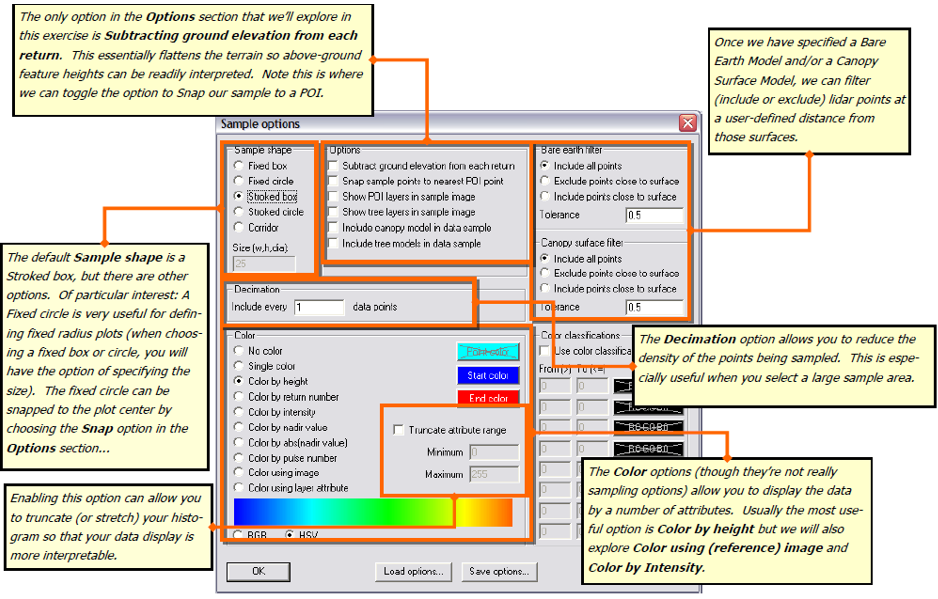
Part 2: Explore FUSION's sampling and display options
Fusion offers a number of ways to sample and view lidar data. We’ll explore several of these options in this section and you’ll use many of the remaining options in later steps.
- Close the LDV Viewer and on the FUSION toolbar (Left Panel), click the Sample options button to open the Sample Options dialog.
- Under the Sample shape section, Select, Stroked circle (the default is Stroked box) and Click, OK.
- Select a small stroked-circle sample (LMB click, hold and drag) in the Fusion window and view the results in the LDV viewer.
- Close the LDV window.
- Return to the Sample options and change the sample shape back to Stroked box.
- In the Decimation section, increase the value to 200 and Click, OK.
- In the Fusion window, select a large window (suggestion: make the stroked box cover about half the size of the reference image.
It may take a few minutes to extract the sample but the results display very fast in LDV. Please notice that the ground is not flat within the sample area as you view the data in LDV—you’ll make it flat in the next step.
- Return to the Sample option and Select (check) the Subtract ground elevations from each return in the Options section and click OK.
- Click the Repeat Last Sample button. This will repeat the last sample area but now the data will appear in LDV on flat terrain—this is very useful for comparing heights above ground level.
- Return to the Sample options and change the Decimation value back to 1 and de-select the option to subtract ground elevations.
- Select the Bare Earth Filter option to Exclude points close to surface and increase the tolerance to 2.
- Click, OK to close the sample options dialog.
- Select a small stroked box sample in the Fusion window. Note that the points close to the ground have been excluded from displaying in LDV.
- Return to the Sample options and Select the Include all points option under Bare Earth Filter.
- In the Sample options window, under the Color options Select, Color using image and Click, OK.
- Click the Repeat last sample button. You should notice that each lidar return is now painted the color of the corresponding reference orthophoto image.
- Click the Sample Options button.
- Enable the Color by Intensity option.
- Click, OK and then Click, Repeat Last Sample. The LDV viewer will display returns according to their intensity value (or the near-infrared spectral value).
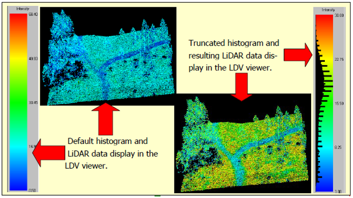
The intensity information can be helpful to interpret ground features. However, because the intensity information of the ground features are clustered on only a small portion of the displayed intensity range, the default display parameters make the data difficult to interpret. Let’s adjust the intensity display parameters to improve interpretation.
- Click the Histogram checkbox on the left side of the LDV viewer (see graphic to left).
- The histogram will display (black) along the color legend.
- You should see that most of the intensity values are clustered in the lower half of the available intensity range. Let’s truncate the available range to the approximate range of the intensity values (so that we can interpret the lidar data better).
- Write down the approximate low and high intensity values that capture most of the histogram (see graphic to left).
- Click the Sample Options button in the Fusion window.
- Enable Truncate Attribute Range (in the Color section).
- Enter your approximate minimum and maximum histogram values.
- Click, OK and then Click, Repeat Last Sample.
Now that you’ve effectively stretched your intensity data to cover the full color legend for improved interpretation (see figure below). High intensity values (or high near-infrared values) for natural features most likely represent photosynthetically active vegetation, and in some cases may represent dry bare soil. Lower intensity values likely represent:
- wet, bare soil,
- water, or
- less photosynthetically active vegetation.
The figure below illustrates how the data and histogram changes with truncation:
- Continue to interact with the data in LDV and experiment with the following items on the right-click menu:
- Wiggle-vision (Alt-W)
- Overhead View (Alt-O)
- Reset Orientation (Alt-R)
- Reset Zoom (Alt-Z)
- Image Plate (Alt-P)
- Turn the truncate function off and choose the color by option that seams most appropriate for general visualization (color by height is recommended).
- Save the project: File | Save.
For more information about sampling options, see Appendix 2
Part 3: Perform simple measurements
- Select a stroked box sample that includes trees.
- Type, Alt+u to display the bare earth model and Type, Alt+i to display the orthophoto on the surface model or access these options from the right-click menu.
You are now able to visualize Lidar points within the measurement cylinder and view the corresponding area of the orthophoto.
- Right Click in the LDV window to activate the pop-up menu and Select, Measurement marker. This will change the display to an overhead view and show the measurement cylinder.
- Move the cylinder by holding down the Shift key and typing with the arrow keys. Move the cylinder so that an individual tree is at its center.
- Resize the measurement cylinder (Ctrl+Shift+Right mouse button + mouse drag up/down) to isolate the crown of a single tree.
- Click and drag the data cloud with the LMB to view the cylinder from the side.
- Press Ctrl and type h to automatically move the cylinder to the highest lidar point. The value of the measurement marker location is displayed in the LDV’s window.
- To measure the ground elevation of this location, press Ctrl and type g to automatically move the cylinder to Lidar points corresponding to the ground surface.
- You can now calculate this tree’s height by simply subtracting the ground elevation from the tree-top elevation.
Another method to make similar measurements is to automatically subtract the ground elevations, let’s do that now...
- Type Alt+i to turn the display of the orthophoto off.
- Likewise, Type Alt+u to turn the display of the bare earth model off (or turn these options off from the right-click menu).
- Return to the Fusion window and Click the Sample Options button.
- Enable the Subtract ground elevations from each return option and Click, OK.
- Click the Repeat last sample button.
Notice that the sample area is “flat” in LDV and the elevation bar to the left is providing Height above ground.
- Right Click in the LDV window to activate the pop-up menu and Select, Image plate (Alt-p) to turn the orthophoto on below the lidar data (you may have to zoom-out to see the image plate if you are zoomed-in).
- Right Click in the LDV window to activate the pop-up menu and Select, Measurement marker.
- Move and resize the cylinder as you did before to highlight a single tree (see side bar).
- Click and drag the data cloud with the LMB to view the cylinder from the side.
- Now, when press Ctrl - h like before, the measurement marker moves to the tree top and gives you the height of the tree (there is no need to type g — in fact, that function is inactive).
- If the height numbers are black and are hard to see with the background, use the right-click menu and Click on the Color.. option and change the Background or Axis color… to a contrasting color (white works well).
Now imagine for a big forest inventory project you wouldn’t want to measure every tree individually like this. In the next part of this lab you will learn to extract fixed radius plot subsets.
Part 4: Extract samples using points of interest
- In Fusion, Click the POI... Button
- Navigate to your “originals” folder and then select “plot_data.shp” shape file and click open.
- Change the attributes (color and size) of the POI if desired (see side bar) and Click, OK.
- Three plot locations will display over the orthophoto.
- Click the Sample options… button (from the menu on the left) and Select the following options:
- Sample shape: Fixed circle
- Sample Size: 50 (diameter in meters)
- Options: Subtract ground elevation from each return
- Options: Snap sample points to nearest POI point
- Click, OK at the bottom left to accept the sample settings.
- Next, within the Fusion display window, Click on one of the plot locations (note which one you select). The POI changes color and an LDV window pops up showing the lidar points within the 50-meter diameter circle around the plot center.

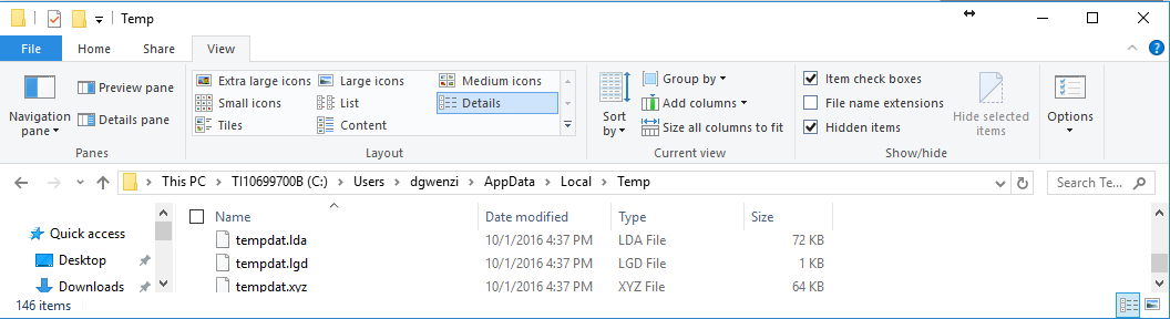
These lidar data points are simultaneously written to three temporary files named tempdat with three different extensions (.lda, .lgd, .xyz) in the user’s temporary folder (e.g. C:\Users\dgwenzi\AppData\Local\Temp) as in the figure below. You might want to check if your folder view options allow you to see hidden files. An easier way to locate the “Temp” folder is by clicking on the windows icon and type %temp% then hit enter.
Potentially you could locate and rename the 3 temporary files with a corresponding plot identifier: for example Plot1.* and move them into a working directory. You would then have a subset (for each plot) of lidar data. It is good to be aware that FUSION writes these temp files and deletes them when FUSION closes (if you want the temp files make sure you move and rename them!)
However, you wouldn’t want to do all this manual work for a big project. In the next section we will work through a process that will allow you to automate the subsetting of many plots and subsequently calculate statistics for each plot. We will now use FUSION command line executables and batch files to accomplish this.
It takes time and effort to create the batch processing scripts so I have prepared them for you (You are welcome!). Using these scripts will give you an idea of how powerful FUSION is and if you want to use its capability in your own work, you will simply have to edit the scripts or consult the user manual to create your own from scratch.
Part 5: Batch processing to extract plot statistics
5.1. Clipdata
This function clips points from a lidar point file that fall within a fixed radius of a point (plot center).
- Navigate to your “codes” folder and open and explore the “clipplots.bat” file with notepad++
Each plot has its own line of code and below is an explanation of the various components of the code:
- clipdata is the FUSION executable command
- /shape:1 denotes a circular shape
- /dtm:C:\Users\dg1688\Desktop\lidarlab\originals\demo_4800k_UTM.dtm denotes the bare-earth surface model used to normalize the LIDAR data (subtract the bare-earth surface elevation from each lidar point elevation).
- /height is used in conjunction with the specified dtm to convert all elevation values to height above ground
- C:\Users\dg1688\Desktop\lidarlab\originals\demo_4800K_UTM.lda specifies the input lidar point cloud data file
- C:\Users\dg1688\Desktop\lidarlab\working\clipplot1.lda defines the output data file
- The last four numbers are geo-coordinates that define the bounding box of the circular shape in the order xmin, ymin, xmax, ymax
- Open the command prompt: Click on the windows icon and then type cmd and then click on cmd.exe or Command Prompt (The option you have depends on your windows version)
From now on you will use the codes that I have prepared for you in your own workspace so before running each code, make sure you replace everywhere it says “dg1688” with your own log in ID
- Now we need to run the “clipplots.bat” script from the “codes” folder. In the command prompt change the directory to the “codes” folder by typing the following (remember to change dg1688 to your own ID):
- cd /d C:\Users\dg1688\Desktop\lidarlab\codes
- Now type clipplots. This will execute the “clipplots.bat” script
- Open your “working” folder and make sure these files are created: clipplot1.lda; clipplot2.lda and clipplot3.lda
Now Let’s look at the plot data in Fusion.
- Ensure that the Image File (demo_4800K_UTM.jpg) and that the three POI’s from above are loaded and visible.
- Click the Raw data… button in the Fusion window.
- If the file demo_4800K_UTM.lda is still loaded, Click on it and then click the Delete button to remove it.
- Click the Add File… button.
- Navigate to your “working” folder and Select, clipplot1.lda
- Hold the shift key down and select the last file, clipplot3.lda, to select all three lidar plot subset files
- Click the Open button.
- Give each data file a different color and change the Symbology. Select one of the rows (each row is a data file) in the Data Files dialog and for each selected row:
- Click the Properties button (or simply double-click anywhere on that row)
- Change the Symbol to Single Pixel
- Click on Line color and then on Fill Color to change them to the same, distinct color
- Click, OK
- Click the check box next to the Raw data… button to display the three lidar subsets. Your Fusion window should be similar to the figure below.

5.2. Cloudmetrics
This function computes a variety of statistical parameters describing a LIDAR data set. Metrics are computed using point elevations and intensity values (when available). CloudMetrics is most often used with the output from the ClipData program to compute metrics that will be used for regression analysis in the case of plot-based LIDAR samples or for tree classification in the case of individual tree LIDAR samples.
The input can be a single LIDAR data file, a file template that uses DOS file specifier rules or a simple text file containing a list of LIDAR data file names. We will use the txt file plotmetrics.txt to extract metrics from the 3 plots we created using the clipdata function above.
- Navigate to your “originals” folder and open the file plotmetrics.txt with notepad ++
- In this text file, change the path C:\Users\dg1688\Desktop\lidarlab\working to match your own working folder
- Save the file and close it
- Navigate to the “codes” folder and open and explore the cloudmetrics.bat file with notepad++
- cloudmetrics – Fusion Command line executable
- id - Switch, use file name to identify output
- new – Switch, creates a new output file and deletes any existing file with the same name
- above:2 - Switch, compute various cover estimates using the specified height break, in our case the height break is 2 m.
- minht:2 - Switch, only use returns above a certain height to compute metrics. By choosing 2 m we will exclude “ground” returns from our output stats. This is a common practice in Forest inventory
- C:\Users\dg1688\Desktop\lidarlab \originals\plotmetrics.txt – Input data specifier, in this case we have used a text file containing a list of the multiple file names, with full file paths included
- C:\Users\dg1688\Desktop\lidarlab \finals\cloudmetrics.csv - Output Data File, this designates the output file name.
- Now we need to run the “cloudmetrics.bat script from the “codes” folder. In the command prompt make sure you are still in the “codes” directory. If not change it like you did before.
- Now type cloudmetrics. This will execute the “cloudmetrics.bat” script
- If your script was executed well, you should have a csv file called cloudmetrics.csv in your “finals” folder
- Open the CSV file and explore the plot statistics
These are the components of the code:
Not only does FUSION calculate metrics for elevation of each return but it also calculates the metrics for intensity if the information is available. At this point in the development of aerial discrete return lidar technology the intensity values are not normalized, so they are not really useful for analytical work. Hopefully in the future this will change and these metrics can be used in more analysis.
Lidar has proven itself, through validated research, to directly and accurately measure height and % canopy cover of forest vegetation. So let’s now take a closer look at our plots to see if we can understand how much the metrics reflect what we see in the field and the lidar point cloud.
Let’s look at the following columns
- Elev minimum
- Elev maximum
- Elev mean
- Elev stddev
- Percentage first returns above 2.00
- Check to see if you got similar results to the ones below:
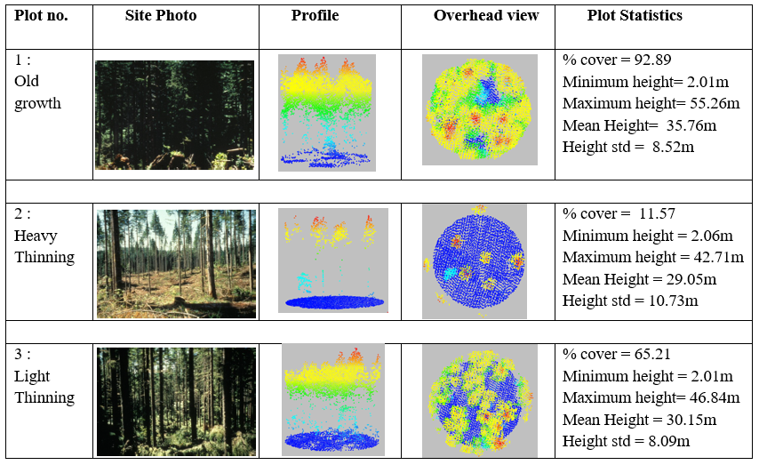
Do these make sense?
5.3. Gridmetrics
The cloudmetrics output is most often used with the output from the ClipData program to compute metrics (just as we did in part 1) that will be used for regression analysis in the case of plot-based lidar samples. The next step would be to explore relationships between field data recorded at the plots and the plot metrics we calculated using FUISION. Once these relationships are established using any number of analysis techniques (linear regression, random forest, etc.….) you can apply the resulting equations across your whole study area. To do this you would need to compute the same metrics you did for the plots across the lidar acquisition. The GridMetrics FUSION command computes the same metrics as CloudMetrics, but the output is a raster (grid) format with each record corresponding to a single grid cell. In this part of the exercise we will compute GridMetrics for the example data set.
- Navigate to your “codes” folder and open and explore the “gridmetrics.bat” file with notepad++
This code has 2 executable lines: - The first line will calculate statistics at 5 m X 5 m cell size and create a csv file “gridmetrics_all_returns_elevation_stats.csv” in our working folder
- The second line extracts data in column 49 of the csv file and export is an asc file to be saved in our finals folder. We can then open this asc file in other GIS programs like ArcMap. Column 49 has the data about canopy cover and in the next step we will use ArcMap to see if this makes sense
- In this text file, replace dg1688 with your own log in ID to make sure the directories match your workspace.
- Now we need to run the “gridmetrics.bat” script from the “codes” folder. In the Command prompt make sure you are still in the “codes” directory. If not change it like you did before.
- Now type gridmetrics. This will execute the gridmetrics.bat script
- When done, open your “finals” folder and make sure the cover_grid.asc file is created
- Open ArcMap
- Click the add data icon and navigate to your “results” folder and select the cover_grid.asc file and click OK. This file may not have Spatial Reference Information. Define it to WGS_1984_UTM_Zone_10N
- Change the symbology of the layer: Use the red-green color ramp to show low canopy cover areas in red and high canopy cover areas in green.
- Now you can overlay the demo_4800K_UTM.jpg file (with about 50% transparency) on top of the cover_grid layer and see if low grid cover layers correspond with open areas in the image
I hope you have enjoyed the lab. For any questions or comments, feel free to contact me:
david.gwenzi@humboldt.edu
Appendices
keyboard Commands
Sampling Options