Lab 11: Visualizing Spatial Data in 3D Along Humboldt Bay

Introduction

The goal of this lab is to create a more realistic and three-dimensional (3D) view of spatial data around Humboldt Bay.

Learning Outcomes

• Use ArcScene to create 3D visualizations of spatial data
• Use bathymetry data to model the ocean floor
• Create "fly-through" animations

Data

DEM of Area Surrounding Eureka

Ortho Image

The data is a DEM of the area around Humboldt Bay (including bathymetry off the coast) and the Ortho Imagery is the same as lab 4 but has been down sampled and saved to a TIFF file for 3d viewing.

Walk Through: Lab Preparation

To set up for this assignment:

1. Create a folder structure in "D:\TempData" as we have done before:
1. 01_Originals
2. 02_Working
3. 03_Final
2. Download the data and decompress it.
3. Check the files and prepare them for work. You'll be working in NAD 83, UTM Zone 10 North.

Walk Through: Preparing Ortho Imagery Data

We need to clip the ortho imagery to just the area of Humboldt County to remove the area of the ocean that is in the image. We'll be replacing this portion with bathymetry for a 3D effect.

4. Load a Humboldt County shapefile. These are available from the Humboldt County GIS Data Download or you may have one from a previous lab.
5. In ArcToolbox, select "Spatial Analyst Tools → Extraction → Extract by Mask". This tool will clip a raster to the area in a shapefile.
6. Select the Ortho raster as the "Input raster".
7. Select the county boundary as the "Input raster or feature mask data".
8. Give the output a good name like "Ortho_Clipped1.img".
9. Now we just need to crop the raster to the area of our Eureka DEM.
10. From ArcToolbox, select "Data Management Tools → Raster → Raster Processing → Clip"
11. Select the "Eureka_DEM" as the "Output Extent."
12. Give the "Output Raster Dataset" a good name and run the tool.

Skill Drill 1: Preparing the "DEM"

All we need to do to prepare the "DEM" is to create a new raster that just contains the areas that are covered with water or the "bathymetry". We'll use the Raster Calculator function, "SetNull()", to to create a raster that has all the pixels that are "out of water" set to "NoData" (i.e. greater than 0) .

13. The "SetNull()" function take two parameters, the first is a condition for the pixels that are set to "null" (NoData) and the second is what to set the other pixels to. The following command will do this:
    1. SetNull("Eureka_DEM.img">0,"Eureka_DEM.img")
14. Save this as "bathymetry.img." as "bathymetry" is what we call elevations that are under the water.

Walk Through: Using ArcScene

ArcScene allows us to visualize spatial data in three dimensions. This can be a powerful way to communicate spatial information to diverse groups. You can also do some 3D analysis but these tools are available in both ArcScene and ArcMap.

15. Open the ArcScene and load the Ortho layer, the "bathymetry" layer, and the "Eureka_DEM".
16. Click on the "Navigating" icon:

17. Press on the layers in the viewing area and move the mouse up and down. You'll see that the layers now appear to be in 3D and you can control how they are oriented.
18. Now lets make our layers look a little less flat and fix the "checkerboard" effect you may be seeing.
1. Select the "Base Heights" tab of the "Properties" for the Ortho layer.
2. Select the "Eureka_DEM" for the "Floating on a custom surface" value.
3. Click "OK."
4. You can also make the "Eureka_DEM" raster invisible now as we are only going to use it for the "Base Heights".

If you look closely, you'll see that there is some change to the image and this is actually a realistic view of the topography around Arcata. However, we really want to exaggerate the topography to make it more interesting.

19. Return to the "Base Heights" tab and enter 5 for the "Factor to convert layer elevation values to scene units". The elevations will be multiplied by this value to exaggerate the elevations. Try other values to see how this changes the topography in the map.
20. Next, we want to make the topography look more realistic.
1. Select the "Rendering" tab of "Properties" for the Ortho layer.
2. Check "Shade aerial features..." in the "Effects" box. This will use the 3D hardware in your computer to render the elevation raster as if it had the sun shining on it, very similar to a hillshade.
3. Repeat the whole of assigning base heights and rendering properties for the bathymetry layer except use the bathymetry layer as the base heights for itself. Then, experiment with different values for the "Factor."
4. You may also want to change the color ramp for the bathymetry to be "blue." You can do this in the "Symbology" tab for the bathymetry layer. You may also want to check the "Invert" option in the "Stretch" box.

By now you may have had one of any number of difficulties with the 3D rendering in ArcScene. ArcScene is not the best product for this and restarting the software might help. It will also work better with better 3D rendering hardware. There are other software packages, including some free ones, that are more sophisticated.

Walk Through: Adding "Water"

One thing that is missing is the surface of the ocean.

30. Return to ArcMap and use the rectangle or polygon, tool to create a rectangle that covers the area of the Eureka_DEM raster.
31. From the "Drawing" drop down menu in the same tool bar, select "Convert Graphics to Features."

32. Set the "Output shapefile" to a file in your working folder and click "OK."

This is a handy trick to create shapefiles that can be used for a variety of purposes, including clipping layers to desired bounds.

33. Load the boundary layer into ArcScene.
34. Set the "Transparent" value in the "Display" tab of the "Properties" for the layer to 50% and give the layer a blue color to make it appear like there is water over the bathymetry layer.

Walk Through: Adding Extruded Values

We can also add vector data and "extrude" it to show values within attributes. Let's add the flood risk and amount of area to the scene.

35. Go to the "Humboldt County GIS Data" download page and download the "Special Flood Hazard Areas" shapefile. Prepare this file for analysis and crop it to the boundary shapefile you created in the previous section.
36. Load the shapefile into ArcScene. Take a moment and look at the data both from above and below. Notice that the data is displayed as "flat" and some of it is under the mountains.

Data can get "lost" in a 3D scene very easily. If you load data and it does not appear, try turning off the other layers and then "zoom to" the layer. Remember that you can also have georeferencing issues in ArcScene just like in ArcMap.

37. Before continuing, create a new field in the "Flood Hazard Areas" shapefile and set it so that high flood risk areas ("A") are a large value such as 10 and low risk areas are a lower value like 0.
38. Go into the "Extrusion" tab in the "Properties" dialog for the flood layer. Make sure that "Extrude features in layer" is checked."
39. Click on the little calculator icon.
40. This "Expression Builder" is similar to Field Calculator. Click on your field with the zone risk values and you'll see it added to the "Expression."
41. Click "OK" and then "OK" again.
42. You'll need to multiply or divide the value to get heights that look good.
43. Return to "Properties" and give the vector data symbology that looks good. you can even make the vector data transparent!
44. Try some other layers for the county such as roads, fire hydrants, and biological zones.
45. Finally, add your homestead polygon shapefile from the previous lab and extrude it so it shows up clearly.

Skill Drill 2: Navigating in 3D

Moving around a map is different in 3D than in 2D. In 2D we can zoom in and out, left and right, up and down. In 3D we can do the same movements plus we can change the orientation of the map. This includes roll, pitch, and yaw; the same directions an airplane can move in. Along the top of ArcScene are a series of tools to control the map. You may already be familiar with moving around 3D scenes in products such as GoogleEarth. ArcScene can be harder to control both because the controls are not friendly and because you do not have the entire world for a reference.

46. Familiarize yourself with the navigation tools described below. Below is a list of the tools in ArcScene. You can do all the navigating you need with the "Navigation," "Zoom In/Out," and the hand tool from ArcGIS.

	Full Extent: this tool is your life jacket to get back to the full view of the scene. I put it here because the other tools can be temperamental and make it easy to get lost in your scene.
	Navigation: controls roll, pitch, and yaw of the scene. Use this tool to position the scene after zooming and moving to the position you want to view it from. Using the left mouse button grabs the layers and rotates them around. Clicking the middle mouse button (wheel) will grab the layers and allow you to move them along the X, Y plane. Clicking the right mouse button and moving the mouse forward or backward will zoom in and out of your data.
	Fly: This tool attempts to emulate the motion of an aircraft. Left click increases your speed, right click decreases it. This can be fun once you get used to it but usually ends up with you get lost in space (remember the full extent tool). Also, the <esc> key will stop your flight.
	Zoom In: Moves the viewing position into the scene. This tool is important but very sensitive.
	Zoom Out: Moves the viewing position out from the scene.
	Center on target: Centers the scene on the point you click on.
	Zoom to target: Can be valuable for animation but you'll want to practice with it.
	Set Observer: Puts the viewer at the point you click on. I don’t recommend this tool for beginners and you'll want to use the "Full Extent" tool to get back to the regular view when you get lost.

Skill Drill 3: Making a Fly-Through

A "fly-through" is an animation that makes it look like you are in an airplane flying through a 3D scene.

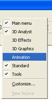
47. Right-click on the menu bar and enable the "Animation" tool bar.

48. Zoom-in or zoom-out to set the viewing position to be where you want to start your animation.
49. Click on the "Capture View" button to record your current/starting position.
50. Move to a new viewing position and click on the Capture View button again.
51. Repeat step 3 until you have added about 5 view positions.
52. Click on the "Open Animation Controls" button
53. Click on the play button in the control window.
54. This will play your animation.

Saving an Animation:
You can save animations in ArcScene to an AVI file or sequential files to create a movie. We want to put our animation onto a web page next week and AVIs are not well supported on the web so we're going to save the movie as "sequential images" and then convert it to a movie in the program "GIMP".

55. Click on the "Animation" menu in the "Animation" tool bar and select "Export Animation...".
56. Create a new folder for the animation.
57. Select "Sequential Images" as the file type and change the "File name" to "Animation1.bmp".
58. When you click "OK" you'll see a dialog appear.
59. Enter "Animation" as the "Filename prefix".
60. Click "OK".
61. After ArcScene is done rendering the images, if you go into the folder you created, you should see a bunch of sequentially numbered "bmp" files.
62. Open "GIMP".
63. From the "File" menu, select "Open as Layers"
64. Select all of the files that were generated.
65. When you click "OK" GIMP will load all the files into a single image with each file being a layer.
66. Select "File->Export" and save the file as a "Filename.GIF" file.
67. Make sure "Animation" is checked.
68. Click "Export". It will take a moment but then GIMP will save a gif animation file.
69. Navigate to the file and double-click on the file to see the movie play.

Addtional Resources

Creating Reports in MS-Word