Raster Analysis - Sea Level Rise Around Humboldt Bay
Introduction
This lab will introduce raster processing by examining the potential impact of sea level rise around Humboldt Bay.
Note: this is a simplified analysis of sea level rise, the real implications of sea level rise, when we incorporate storm surge, tsunamis, and tidal variability, will actually be worse.
There is additional information and maps available at:
Learning Outcomes
- Be able to use the following ArcGIS tools in spatial analysis:
- Resample
- Raster calculator
- Polygon to raster
- Reclass
- Be able to describe the basic advantages between raster and vector data types.
Data
DEM for Humboldt County
The DEM is from the National Elevation Data set and has been mosaicked together from a number of TIFF files from the National Elevation Data set.
Walk Through: Lab Preparation
Before you begin, take a moment to remind yourself about the file and directory naming restrictions in ArcMap, it gets more tricky and frustrating with Raster Analysis tools. Pay attention to the reminders below to make this lab much smoother for you.
- DON'T run your analysis off a network drive such as the G:\ drive
- Folder names: No spaces for all the directories and subdirectories
- File names: Limit the number of characters to 8 and the name should contain only numbers and letters of the alphabet
- Punctuation marks are not allowed
- Special characters are not allowed, except for underscores
- If you have intermediate files before the final product, we recommend ending the filenames with a number e.g slope1
- ArcMap has a seperate tool called "Project Raster" for changing the SRS of raster files. Refresh yourself about the difference between "Define" and "Project".
- The properties you set when creating a new field for an attribute table will determine the type of data you can enter. Refresh yourself about:
- Numeric vs Text
- Short interger vs Long interger
- Float vs Double
To set up for this assignment:
- Set up your standard workspace for this project within a parent folder and 3 sub-folders: Originals, Working, Final.
- Download the data into the "Originals" folder, unzip it, and make sure the spatial references are defined correctly.
- The spatial reference system for this lab is "North American Datum 1983, Universal Transverse Mercator Zone 10 North" or "NAD 83, UTM Zone 10 North". Copy data sets that are in this spatial reference from the "Originals" folder to the "Working" folder and "Project" any data sets that are not in this spatial reference to the "Working" folder.
You'll want to download the DEM for Humboldt County from the link above. This DEM has been cropped to the area around Humboldt Bay to make the raster processing steps in this lab go faster.You may want download an outline of Humboldt County at this time and use the "Extract by Mask" tool in ArcGIS to remove the large "blocky" areas in the ocean. You can also do this as a final step while making your maps.
Walk Through: Creating models for various levels of sea level rise
Like many tasks in GIS, once we have the data setup correctly, doing analysis flows relatively easily. Here, we will create rasters representing the land that might be inundated by water as the level of the ocean rises. I say "might" because there are other factors such as dikes that will be missed by this analysis.
Take a look at the flow chart below as this lab does not use many tools in ArcMap but there are a number of data sets to keep track of.
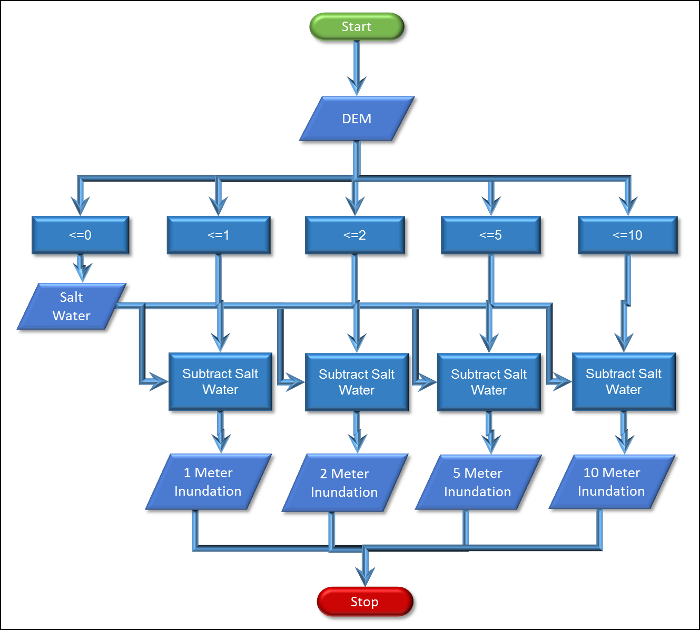
- Open the "DEM" in ArcMap.
When you open raster files, ArcMap will typically ask if you want to create "Pyramids" unless they are already available. You'll want to say "Yes" if you are going to use the raster data repeatedly as this will greatly speed up the rendering of raster data.
- To check the spatial reference for a raster, you need to scroll down in the "Source" tab in "Properties" as it is toward the bottom.
- At the top of this list are some very important information about the raster.
- Columns and Rows: Number of pixels horizontally (columns) and vertically (rows)
- Number of Bands: 1 for most rasters, 3 for RGB (one for red, one for green, one for blue)
- Cell Size (X,Y): the width (X) and height (Y) of each pixel in the raster in the units defined in the spatial reference
- Uncompressed Size: The size of the raster if it was all loaded into disk at one time
- Format: File format
- Pixel Type: floating point or integer
- Pixel Depth: 8-bit, 16-bit, 32-bit, and 64-bit.
- NoData Value: This numeric value is used to represent "no data" or null values. Pixels that are not valid will be set to this value and will appear transparent.
The data types have different names from the ones for attributes. In the table below, first column gives the names of the data types you'll see in some of the tools in ArcMap such as "Create Raster Dataset.". The first part of the name indicates the number of bits used for each sample in each pixel of the raster and the remaining part of the name gives additional information on how the samples are stored (32_BIT_UNSIGNED means the sample is 32-bit in length and is an unsigned integer).
| Pixel Name |
Type |
Attribute Name |
Minimum |
Maximum |
Precision |
| 1_BIT |
Integer |
- |
0 |
1 |
<1 digit |
| 2_BIT |
Integer |
- |
0 |
3 |
<1 digit |
| 4_BIT |
Integer |
- |
0 |
15 |
1 digit+ |
| 8_BIT_UNSIGNED |
Integer |
- |
0 |
255 |
2 digits+ |
| 8_BIT_SIGNED |
Integer |
- |
-127 |
127 |
2 digits+ |
| 16_BIT_UNSIGNED |
Integer |
- |
0 |
65535 |
4 digits+ |
| 16_BIT_SIGNED |
Integer |
Short Integer |
-32767 |
32767 |
4 digits+ |
| 32_BIT_UNSIGNED |
Integer |
- |
0 |
4294967296 |
9 digits+ |
| 32_BIT_SIGNED |
Integer |
Long Integer |
-2147483648 |
2147483648 |
9 digits+ |
| 32_BIT_FLOAT |
Floating Point |
Float |
Big negative number |
Big positive number |
7 digits+ |
| 64_BIT |
Floating Point |
Double |
Huge negative number |
Huge positive number |
15 digits+ |
Question 1: List the "Pixel Type," "Pixel Depth," and "Cell Size" for the DEM.
- In the Toolbox, select "Spatial Analyst Tools → Map Algebra → Raster Calculator." This is a powerful tool that allows you to "do math" on entire raster images as if you were just doing math on a regular calculator.
Chances are you will get the following error:
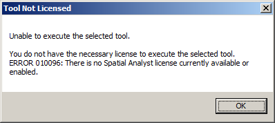
Since "Raster Calculator" belongs to a special extension within ArcMap, we must first turn on the extension to use its functions. Choose "Customize -> Extensions… ->" Then check the box next to Spatial Analyst.
Raster Calculator is similar to the field calculator. On the left is a list of the raster layers you have open in ArcMap. On the right is a list of the "functions" that you can apply to rasters and in between these two are numbers and "operators" that you can use to operate on two rasters to produce a new raster.
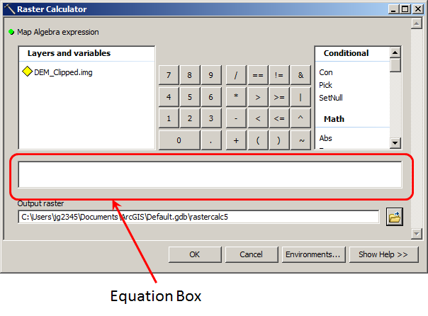
- Double-click on the DEM to have it added to the equation as you did in the Field Calculator. Then click on "<=" and then "0" to find the elevations that are at or below sea level.
- Give the new raster an appropriate name like "MSL_2010.img." Make sure it ends in ".img" for the "IMAGINE" file format and click "OK". The new raster should appear and you should be able to see the outline of the existing Humboldt Bay.
- Take a look at the legend and you'll see that there is "0" and "1." Raster Calculator has created a new raster that contains 0s where the equation you entered was "false" and 1s where the equation was "true." This is a powerful tool to create new rasters that contain the areas you are really interested in for different types of analysis.
- Repeat the process above for areas that are less than one or equal to 1 meter and give the output raster a convenient name like "Below_1m.img". You now have one raster that contains 1s for everything at or below zero meters and one that has 1s where everything is at or below 1 meter.
- Let's subtract the "MSL_2010.img" raster from the "Below_1m.img" raster to find the areas that are above zero meters (sea level) and below 1 meter in elevation.
- Subtract the sea level raster from the raster with elevations below or at 1 meter in the "Raster Calculator" and save it to a new raster conveniently named to something like "Flood_1m.img". The equation for this step should be: "Below_1m.img" - "MSL_2010.img". This step will create a raster showing the area that will be flooded or "inundated" by the ocean if the sea level rises by 1 meter.
- Take a look at the raster you just made. Cell values will be 1s where the elevations are between sea level and 1 meter and 0s everywhere else. This raster will theoretically show the area of land that will be covered by water or "inundated" if we have a 1 meter sea level rise.
Question 2: How much land appears to be between 0 and 1 meters? You may need to zoom in and toggle between the two layers to see the pixels that are between 0 and 1.
- The problem with the image above is that the ocean level moves up and down and there really isn't a "0" elevation. "Mean Sea Level" has been selected as the 0 elevation but this actually varies quite a bit over time and in different regions. Local data is required to improve these estimates and this becomes very involved, we're going to continue with this dataset to see what we can learn for higher elevations.
Skill-Drill: Additional Sea Level Rise Rasters
- To have a more interesting model, repeat the steps above to produce rasters that show the potential areas of inundation for 2, 5 and 10 meters. To do this, you'll want to first create rasters that show the pixels at or below the desired elevation (i.e. 2, 5 and 10 meters), and then subtract the sea level raster from those rasters.
When completed, you should have a series of rasters that have pixels with "1"s where the sea will inundate the land for 1, 2, 5, and 10 meters of sea level rise..
Walk Through: Creating a land use raster
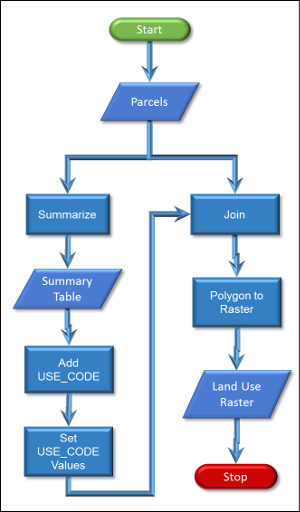
- To evaluate the impact of sea level rise, we need some data on the various land uses in the Humboldt Bay area. In other words, the impact of sea level rise on an a residential area would be very different from an area of range land.
- Download the "parcel" shapefile here: Humboldt County Parcels (this is an older version of the shapefile that contains a "LandUse" attribute that matches the steps below).
- Un-compress, define, and project as needed. Remember only to "Define" if the spatial reference is missing or incorrect and then "Project" the data to the spatial reference you are using for this lab.
- Load the data in ArcMap and you'll see that it covers the entire county and contains a number of attributes including the type of land use (column "EXLU4").
- We can reduce the number of values in the "EXLU4" column to make it easier to use the data. Right click on the attribute "EXLU4" and select "Summarize...".
- This tool will create a summary of all the values in an attribute field. You can leave the settings for "1." and "2" as they are and then make sure the "Specify output table:" setting is going to save a dBase, or "dbf", file into your "Working" folder. "dbf" is an old file format for tabular data that is the same format that is used for attribute tables.
- When you click "OK", ArcMap will create the summary table and add it to the "List by Source" option in the "Table of Contents".
- Tables in ArcMap work just like an attribute table and you can right-click on the table and select "Open" to edit the contents of the table.
- We need to group the large number of categories in the EXLU4 table into a smaller number of categories and covert them to numbers so we can use them in a raster. So, add another integer attribute/field to this the new table, call it "USE_CODE", and give each of the rows an appropriate numeric value as below.
- City
- Agriculture: include timber production
- Residential all categories of "residential"
- Commercial all categories of "commercial"
- Industrial: all categories of "industrial" and mining
- Recreational: include camp, golf courses, open space
- Tribal
- Public
- Other: all others including blanks
You will need to start and end an "Edit" session to type into the attribute columns.
- The next step is to "Join" the new table back into our original table.
- Right click on the parcels layer "Joins and Relates -> Join..."
- Select "Join Attributes from a table" in the "Join Data" dialog.
- Select "EXLU4" as the field for item "1."
- Select your summary table as the "table to join to" in item "2" and the "EXLU4" as the field.
- You don't need to worry about the "Join Options" because all of the records will match. Click "OK"
- Return to the attribute table for the parcel data and you'll see the new attribute for land use type has been added with the new values.
- This joining is temporary, thus it will disappear once the file is closed or ArcMap restarts. To make it permanent, export the current parcels layer to a new shapefile and give it an appropriate name. By now you should know how to perform this export in ArcMap.
- To avoid confusion, remove the old parcels layer from the table of contents and keep only the new layer, i.e. the one you have just created in the export above.
- Now we want to convert our polygon land uses to a raster so we can compare it to our sea level rise rasters:
- From the Toolbox, select "Conversion Tools -> To Raster -> Polygon to Raster".
- Specify the parcels layer as your input features.
- Stop for a moment and think about why we are doing this polygon to raster conversion. This will help you specify the correct "Value field". If you use the default or specify the wrong field, you will have a wrong output raster. In this case we need an output raster of our new land use codes so select this attribute for the "Value field".
- Give the output raster file an appropriate name that ends with ".img".
- Specify the "Cellsize" to be the same as our DEM. You'll want to copy it from the "DEM" raster properties.
- When you click "OK" a new raster should be added to your map that contains the land use type in each pixel based on the polygons that overlap with the raster. Check the attribute table to see if your new values appear.
Question 3: Zoom in to an area of Arcata and examine the differences between the raster and polygon version of the parcel layers. What impact do you think this difference will have on the analysis?
Question 4: What "Pixel Type" is the new raster?
Skill Drill 1: Finding the change in areas of inundation
For the final step, we'll be computing the amount of area of each land use type that could be inundated by different levels of sea rise.
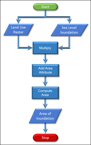
- Our sea level rise rasters contain 1s where there will be sea level inundation and 0s (or null values) elsewhere. Because of this, we can just multiply this raster by our land use raster and we'll just have the land uses where there will be inundation by sea water.
- Multiply the 1 meter inundation raster by the parcel raster using "Raster Calculator".
- Examine the new raster and you'll see that it contains non-zero values only where there will be inundation.
- If you open the attribute table for the new raster, you'll see the "Count" field. This is the number of pixels that contain each land use value.
- Create a new field in the attribute table for the "Area" of inundation for each land use type and then use Field Calculator to compute the area in hectares. A hectare is 100x100 meters (10,000 meters squared), and the pixels are 8.964 x 8.964 meters or about 80.35 meters squared.
- To complete this step, you'll want to remember back to algebra when you did unit conversions. First, we'll convert the number of pixels to meters squared by multiplying the number of pixels times the width of the pixel in meters and then multiplying by the height of the pixel in meters. Since the height and width are 8.964, we obtain the equation:

- We can simplify this equation to:
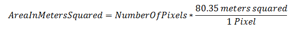
- Then, we'll convert the AreaInMetersSquared to the area in hectares.

- We can combine the second and third equations by substituting for AreaInMetersSquared to obtain:

- By dividing 80.35 by 10,000 and canceling out the units where they appear on the top and bottom, we arrive at the final equation that we can type directly into field calculator:

- So, to convert pixels to hectares you can just multiply the number of pixels (i.e. Count) by 0.008035.
- Repeat this for the 2, 5 and 10 meter inundation rasters.
- Create a table that shows the hectares of different land uses that could be inundated by different levels of sea rise. It will probably be best to make the sea level rise the columns (1, 2, 5, 10) and the rows the different land use types.
Walk Through: Creating an inundation risk map
We also want to create a map that shows the various levels of sea rise.
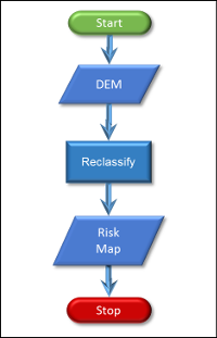
- In the toolbox, select "Spatial Analyst → Reclass → Reclassify." This is a tool that lets you change the values in a raster based on ranges of values or individual values.
- Select your original "DEM_Clipped" raster for the "Input raster."
- For multi-band rasters, you'll need to select a "Reclass field" but since this raster only contains one band, you don't need to change this setting.
- Click on the "Classify..." button. You may receive an error at this point because the raster is floating point instead of integer. This is OK and you can proceed.
- In the dialog that appears, select "6" for the number of "Classes."
- Select "Manual" for the method as we want to specify our own ranges of values.
For some reason, once you select "Manual," you cannot change the number of "classes" so you have to change this value first.
- Click on each of the "Break Values" on the lower right and enter the values 0, 1, 2, 5, and 10 as below. Leave the last value as the maximum value in the raster or you will receive an error.
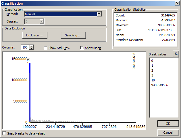
- Click "OK" and you'll see the "Break Values" appear as in the "Old values" column. This shows that the "old values" in your "Input raster" will be "reclassified" to the "New values" on the right of the "Reclassification" box.
- Click on the "New value" for the first row and change it to "NoData". This will make the pixels at or below sea level transparent.
- Do the same with the other "New values" so they match the image below
- Check the "Change missing values to NoData (optional)" box (see below).
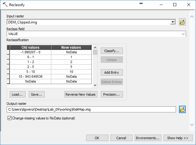
- Click "OK" and you should now see a new raster appear that has separate sections of pixels for each of the potential levels of sea rise.
- Click on the colored boxes next to each different entry to give it an appropriate color. You might make the pixels that are within 1 meter of sea level red to show they are at greater risk and those at 10 meter green to show less risk. You'll also want to change the numbers to appropriate text for your legend.
Reclass Confusion (optional)
The "Reclassify" tool sometimes creates confusion over how it will reclassify values. As an example, take the dialog below where we are going to reclassify a raster. What is going to happen to a value like "2", will it become a "1" or a "2". The way to think about how it works is that the tool starts at the top and if a value matches the "Old value" (in this case, is equal to 2), then the tool will replace the old value with the new value ("1") and move on to the next pixel.
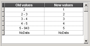
This dialog should really look like:
| Old values |
New values |
| Equal to 2 |
1 |
| Greater than 2 and less than or equal to 3 |
2 |
| Greater than 3 and less than or equal to 4 |
3 |
| Greater than 4 and less than or equal to 5 |
4 |
| Greater than 5 and less than or equal to 943 |
5 |
| Equal to No Data |
No Data |