Lab 7: Research Sites, Part 2 - Creating Streams and Watersheds

Introduction

In the previous lab, we learned where to acquire data and how to perform a standardized quality assurance and quality control procedure. Now that we have the data, we will prepare it for analysis by projecting the data into the same projection and coordinate system. Once this is done, we will create some additional data sets and run some basic calculations.

The key questions we are trying to ask with this lab are:

How many streams are there in Arcata Forest and what is their total length?
What are the watersheds in Arcata Forest and how large are they?

Learning Outcomes

Use the " Project " tool to project data into the same spatial reference
Create stream networks and watersheds from a DEM
Use Raster Calculator for simple raster math.
Create fields (attributes) and compute length and area.
Create maps that convey results of spatial analysis

Clipping The Wetlands Data

One of the layers we want to look at are the wetlands for California but the data set is huge! If you have not done so already, "clip" it to just Humboldt County.

In ArcGIS Pro, select the "Analysis tab"
Click on the "Clip" tool
For the "Input Features" use the "CA_Wetlands" shapefile (depending on the downloaded file, it may be "CA_Wetlands_North").
For the "Clip Features" use the Humboldt County Boundary.
Set the "Output Feature Class" to "Humboldt_WetLands.shp" and save it in the "Humboldt_County" "Originals" folder.
When you click "OK", ArcGIS will take a few minutes and then should display a wetlands shapefile for just Humboldt County that will load and redraw much faster than the one for all of California.

Walk Through: Projecting Vector Data

It is important that each layer in any analysis you perform have the same spatial reference system. This will minimize uncertainty and error. Any error related to map projections will at least be uniform throughout the analysis if they all share the same spatial reference system.

In this step we will project each of our data sets into WGS84 UTM Zone 10 North. This is an international coordinate system based on the Transverse Mercator projection. It is particularly accurate for regions with a North/South orientation, such as Humboldt County. UTM always uses meters as the linear unit.

Using the folder structure from the last lab, download the Arcata Forest data and add it to your "1_Originals" folder. I have checked these data sets and they are all in "NAD83_StatePlane_California_I_FIPS_0401_Feet" and appear OK except that some of them cover a larger area than just the forest.
Also, download the Humboldt County parcels and roads layer (or copy them from a previous lab).
Create a "2_Working" folder next to your "1_Originals" folder.
In ArcGIS Pro, select the "Analysis" tab, click on "Tools".
Search for "Project" and select the "Project" tool.
Select the clipped "CA_Wetlands" data set for the "Input Dataset"
Save the output data set to your "2_Working" folder and give it a good name such as "Humbolt_County_Wetlands.shp"
Make sure to set the "Output Coordinate System" to WGS 84, UTM Zone 10 North
Repeat this process for the following data sets (note that the names of the original files may have changed):
1. apnhum53sp.shp -> Humboldt_Parcels.shp
2. humtrans3sp_20130417.shp -> Humboldt_Roads.shp
3. From the Arcata Forest data set:
  1. cfroads83v7 -> Forest_Roads.shp
  2. creeksp83v13 -> Forest_Creeks.shp
  3. cftrails83v8.shp -> Forest_Trails.shp (I believe this is "version 8" but I did not see any differences between this an "v7")
  4. ACF_boundarysp83v3.shp -> Forest_Boundary.shp
  5. waterbodysp83v10.shp -> Forest_Waterbodies.shp

Once the project tool is complete, you should see a copy of each of these layers in your "2_Working" folder.

Ready for Analysis?

When completed, you should have folders in your "2_Working" folder that contain data for Humboldt County and Arcata Forest. All the data should be in the same spatial reference and ready for us to do some Spatial Analysis!

A great thing to do before proceeding is to go to "Project -> New", create a new map, and then load all your files from the "2_Working" folder into the program. You should not receive any warnings or errors. If you do, something went wrong and you'll want to fix it before proceeding.

Streams Data

Streams data is very important to natural resource research but it is also very challenging to find a "good" stream layer, especially at high resolution. In this step, we'll take a look at some existing stream layers and then create one of our own.

Comparing Water Body Layers

In your GIS application, load the data sets for:
1. Arcata Forest Boundary
2. Arcata Forest Creeks
3. California Wetlands that were clipped to Humboldt County
Zoom in to the layers and take a minute to examine the layers.

The bottom line is that none of the water body layers we have are going to work for the research we want to do in Arcata Forest. Because of this, we need to create a new stream layer. I recommend walking through these steps rather carefully as a wrong turn can cause your computer to crash or take a really long time to finish processing.

Finding Watersheds in ArcGIS Pro

Clipping a DEM

First, to make the stream network processes move fast, we need to clip a DEM to just the area around Arcata Forest.

Create polygon shapefile and then create a rectangle that represents the data you want to clip the raster to. Because we will be making watersheds that include area around the forest, make sure to leave a large buffer by making the polygon about 3 times the width and height of the forest. Make sure to save your edits.
Clipping rasters is different from clipping vectors so open the search box and type in "Clip Raster"
The first item should be "Clip Raster" in "Data Management". Select this tool.
Select the DEM from last week that overlaps with Arcata Forest as the "Input Raster" and the clipping boundary" as the "Output Extent". Then, set the "Output Raster" to "DEM_Clipped.img" in your Arcata Forest working folder.
The clipped DEM should appear around your Arcata Forest boundary.
You can now remove the larger DEM from ArcGIS.

Walk Through: Projecting Raster Data

To project a raster to a new spatial reference, we need to use the "Project Raster" tool.

In Geoprocessing search for "Project" and select "Project Raster".
Select the "DEM_Clipped.img" for the "Input Raster"
For the "Output Raster Dataset" be sure to save to your working folder. Call the output "DEM_Clipped_Projected.img". The "img" or "Imagine" file format is the best file format for rasters when working with ArcGIS.
For the "Output Coordinate System", open the Spatial Reference Properties window by clicking the icon on the right. Just as before, we can use the "Layers" folder to select "WGS_1984_UTM_Zone_10N".
Select "BILINEAR" for the "Resampling Technique" or you will have artifacts in your DEM that will show up when you create direction or hillshade rasters from it.
Leave the remaining default settings as they are and click OK.
The result will not look any different because ArcGIS projects all layers "on the fly" to the spatial reference set in the "Map" properties.

Note: ArcGIS Pro gave me an unknown error when I tried to project the DEM to UTM so I projected it in BlueSpray. QGIS might work as well.

Checking for Artifacts and Creating Hillshades

Before continuing, we want to make sure our DEM does not have any artifacts that could cause problems (this happens a lot with DEMs). A handy tool for this, and making backgrounds on maps is the "Hillshade" tool.

In Geoprocessing, search for "Hillshade".
1. If you receive an error that you do not have a license for these tools, go to "Project -> Licensing" and click on "Configure your licensing options". Use this dialog to turn on licensing for Spatial Analyist to access the Hillshade and other tools.
Select our clipped and projected DEM for the "input raster"
Give the "Output raster" a good name like "Hillshade.img" and save it in the Arcata Forest working folder.
For now, we'll leave the "Azimuth" and "Altitude" values at the defaults as these are also the default for most western maps.
When you click "OK", you should see a simulation of light reflecting from the topography as if the sun were to the north west. If you see any lines running through the hillshade that should not be there then you have "artifacts" in the image from processing or the original data collection and you'll run into problems down the road.
Hillshades are very commonly used for backgrounds on maps as well. As long as we're here, let's make one.
In ArcGIS Pro,
1. Right click on your DEM and select "Symbology".
2. Change the "Color scheme" to something interesting.
3. Click on the "Appearance" tab and use the slider at the top of the "Effects" box to change the transparency to 50%.
4. If you do not see a colorized hillshade, make sure the DEM is above the hillshade in the Table of Contents.
Zoom into the hillshade and look for artifacts that might cause problems when making a stream network. You might see what looks like indentations along the ridge lines. What impact might these have?
When you have a chance, come back to these steps and play with the color ramps and other settings to make nice backgrounds for this report and future ones.
Note: Change the "Brightness" in the "Display" tab of both rasters to make the hillshade fade into the background.

Creating a Stream Network

Creating a stream network requires a number of steps but should work out if you are careful (or are ready to go through the process several times).

Load the DEM that is clipped around Arcata Forest from the previous section.
In Geoprocessing, click on the "ToolBoxes" tab and go to: "Spatial Analyst Tools" -> Hydrology". Typically we just search for tools but all the Hydrology tools are in one toolbox so they are easier to access this way.
Before we work with a DEM we have to "Fill" any "Holes" in the DEM. These are pixels that have very low values and will cause a stream to disappear during processing (take a look at your existing streams layers and see if you can find the one that was done with a DEM without the holes filled). Select the "Fill" tool.
Select our clipped and projected DEM for the "Input surface raster"
Name the "Output surface raster" "Filled.img" and save it into the Arcata Forest working folder. When you click OK, you should see a new DEM that looks just like the old one.
The next step is to create a raster that shows the direction that water will flow downhill. Select the "Flow Direction" tool.
Use our filled DEM for the "Input surface raster"
Set the "Output flow direction raster" to "Direction.img" and save it into the Arcata Forest working folder. you should see a very brightly colored image where the pixels have been given "codes" for the cardinal direction (N, NW, W, SW, S, etc.) for the direction that water would flow from this pixel.
We'll now use the Direction raster to create a raster where each pixel represent the number of pixels that "flow" or "accumulate" into it. Select the "Flow Accumulation" tool.
Select the "Direction" raster for the "Input flow direction raster" and give the output raster a name like "Accumulation.img" and save it in the "Arcata Forest" working folder.
After you click "OK", you should see a few lines that are the ends of the streams that appear in the DEM. To see these better:
1. In ArcGIS Pro:
  1. Right click on the "Accumulcation" layer and select "Symbology"
  2. Make sure the "Primary Symbology" is "Stretched"
  3. I find that the "Stretch Type" of "Histogram Equalization" is the best to see all the accumulation paths.
Do you notice anything strange about the accumulation of water in the raster?
Next, we need to create a raster that contains 1's where we want the steams to be and 0's elsewhere. In Geoprocessing, search for "Raster Calculator". This is a powerful tool that lets you do mathematical and other operations on entire rasters. Double click on the "Accumulation" raster and then type ">100".
Name the output file "Accumulation_GreaterThan_100.img" as on a real project, you would probably try different amounts of accumulation.
When you click "OK", you should see a raster with 1's where the pixels along the streams have "accumulated" the water from over 100 other pixels.
Try one at 1000 pixels and some other values. Note that this tool is handy for making streams at different levels of detail for research and for cartography.
Our last step is to convert these rasters to polylines that represent a stream network. Open the "Search" tool and enter "Raster to Polyline".
Use your Accumulation_GreaterThan_100" raster for the "Input rater" and name the output "Streams_Over_100.shp". Make sure to turn off "Simply polylines"!

Clean up

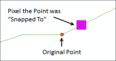
You may have noticed some little squares where the conversion to polyline followed multiple paths for your streams. These are not desired so we'll need to remove them.

Clip the streams to just the boundary we used for clipping the DEM (i.e. a boundary larger than the forest boundary) and use the new stream shapefile for this section.
Open the attribute table.
Start and edit session.
Zoom in to one of the areas with the extra polylines.
Select some of the extra polylines.
At the bottom of the attribute table window, select the icon to "Show selected records". This will allow you to view just the selected records and you should now see the rows for the features you selected.
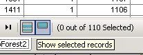
Right click on one of the rows and select "Delete Selected".
The rows should disappear and the extra polylines with them.
Repeat this process until all the extra polylines within the forest are gone and then, stop the edit session.
You also may have noticed that the stream reaches are broken into far more segments than needed. Run the "Unsplit" tool to join the streams into their correct reaches.

When completed, you should have a stream network that is a visible improvement over some of the other layers and, even more critically, it matches your DEM exactly for future analysis!

Comparing Results

Load your other water body layers into ArcGIS Pro and compare them with your new stream layer. Add a map for this new layer to your report.

Finding the Watershed

Using our direction raster we can create a polygon shapefile that describes the "watersheds" in our area of interest. First, we need to create a point file that contains "pour points". These are the points where the water will "flow" through the streams. ArcGIS uses these as a starting point and will then backtrack using our direction raster until it reaches the ridges that define our watersheds.

Create a point shapefile as we have done before (right click on the folder in ArcCatalog, select "New Shapefile", etc.).
Name the file "PourPoints.shp".
When you create the file, make sure to set the spatial reference to match your existing layers.
When digitizing your points, make sure to zoom in and the tool should "snap" to your polyline for your stream.
Your selection of points is also important. Try to find areas of stream reaches that are away from tributaries and low in the watershed. This will reduce the number of points you need.
Make sure to "Stop Editing" when you feel you have a good set of points.
Before creating the watershed, we need to make sure our points are actually on the accumulation raster pixels that the stream flows through.
Open the "Hydrology" tool-set in Spatial Analyst and select "Snap Pour Point". This feature will create a raster with pixels that are in exactly the location we need.
Select your pour point shape file for the first input.
Select the "FID" as the "Pour point field" so we have a unique value for each pixel in the watershed.
Select the accumulation raster you made above for the "Input accumulation raster".
Give the raster a good name and save it in your working folder.
The "Snap distance" is how far ArcGIS should look for the highest value (our stream course) in map units (i.e. meters). Enter a value that is a few pixels across (if you've forgotten the resolution of our rasters, you can check in "Properties -> Source".
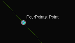
Zoom into one of your pour points and you should see a pixel nearby. Grab the "Info" tool and check that the pixel value matches the FID of the point nearby.
Finally, select the "Watershed" tool from the ArcToolbox.
Select our direction raster for the first input.
Select the "pour point" raster you just created for the second input.
Give the watershed output a good name and save it in the working folder.
When done, you should see watersheds for Arcata Forest. However, don't be surprised if this does not work the first time. You will probably have to go back to step 7 and add pour points or move them to be on top of the right accumulation pixel to catch all the watersheds.

Warning: Do not create multiple files with pour points and then try to merge them together. The watershed tool relies upon a single set of pour points to accurately determine the watersheds.

Finding the watersheds and stream network in BlueSpray

BlueSpray is availabe on the lab computers or at the BlueSpray website. There are technical difficulties with Java applications on the Cal Poly Humboldt campus and ITS is working on resolving these. In the mean time, they have installed and tested a copy of BlueSpray on the GIS lab computers that should work for the following steps.

This video shows the process of creating watersheds and stream networks in BlueSpray.

Clip the raster to the area of interest

Load the DEM by dragging the DEM file into a view in BlueSpray
Drag and drop the forest boundary shapefile into BlueSpray. BlueSpray will let you know if the data needs to be reprojected and then will reproject it to match the DEM
Use the Marquee tool to select the area to crop. You will want to leave quite a bit of space around the forest to make sure you get all of the watersheds.
Right click on the DEM layer and select ”Transforms General -> Crop Raster”.
Select AOI in the "Set To" popup to set the cropping bounds to the area of interest you defined.
Click OK to crop the raster to the selected area. This will create a new layer.
Right click on the old DEM and select “Remove”
Right click on the new DEM layer and select “Export to File…” to save a copy of the DEM
Note that BlueSpray keeps everything in memory, not on disk. This makes processing very fast but dangerous! Remember to save any layers you need.

Projecting the DEM

If the DEM is not in the desired Spatial Reference System (SRS, aka Coordinate System and sometimes incorrectly referred to as a projection).
Right click on the “Scene” and select “Transforms -> Change SRS”. If this is grayed out, it is because you don't have a defined SRS and you’ll need to “Define” one first.
Select your desired SRS.
BlueSpray will project all the data in the scene to the new SRS.
Save the new DEM if desired.

Checking for Artifacts

Right click on a DEM in BlueSpray and select "Transforms: Cartography -> Carto Mixer". This is a tool that makes it easy to create hillshades (AKA shaded reliefs).
Click on the "Update" button to see an initial, gray-scale, shaded relief.
Click in the "Color Ramp" popup and select a more colorful ramp and then select "Update". A more colorful ramp will make it easier to see artifacts.
When you have a color ramp you like, click "OK".
Zoom into the image and see if you can find any systematic patterns in the DEM. This is a major problem because the water will flow along the patterns rather than follow the true water course.
The Carto Mixer creates RGB rasters that can be saved as TIFF files and then loaded into your favorite cartography package as backgrounds.

Finding the initial Direction Raster

Right click on the DEM (not the hillshade) and select “Transforms: Water -> 2. Find Flow Direction”.
Make sure the DEM is selected as the first input and click OK. The resulting Flow Direction layer will be displayed with arrows to show the direction of flow. Circles are used for one pixel sinks. Squares represent two or more pixels that have the same value and are thus “flat”.

Making all the pixels flow to a pour point

The steps below will create a direction layer that does not have any flat areas and only has sinks on the edge of the raster. Follow the steps carefully and make sure the right layers are specified in each of the transforms or things can go wrong!

Finding the Pour Points

Right click on the Original DEM and select “Transforms: Water -> 3. Find Pour Points”.
Click OK. This may take a few minutes for large rasters.
The resulting Pour point layer may contain a large number of pour points. This is because all the little watersheds at the edge of the raster each get a pour point. You actually want all these because it keeps the water on the edges flowing off the raster instead of into your watershed.

Finding the initial watershed raster

Right click on the Pour Point raster and select “Transforms: Water -> 4. Find initial watershed raster”.
Make sure you have the correct pour point and direction raster selected and click “OK”. This transform will flow all the pixels in the specified direction raster into the provided pour points. Each pixel that is found to be in a watershed will be given a value that is greater than 0 to identify the watershed it is in. Pixels that do not make it to a pour point, will appear with a value of 0. For most DEMs, the large majority of the pixels will not flow to a pour point. The next steps will address this.

Finding the rest of the watershed

Right click on the watershed raster and select “Transforms: Water -> 5. Add Pixels to Watershed Raster”.
Use the watershed raster that was created above and the same direction and elevation raster and click “OK”. This transform will then add the pixels with a value of 0 to a watershed raster. This is done by “filling” sinks and flowing “flat areas” into the appropriate watershed. This will produce a new direction raster with all pixels flowing to a pour point.
Note that this is one of the few BlueSpray transforms that modifies an existing raster rather than create a new one.

Find the accumulation raster

This step will create an accumulation raster where each pixel is a count of the number of pixels that flow into it.

Right click on the "Flowing Direction Raster" and select “Transforms: Water -> 6. Find accumulation”.
Accumulation rasters contain very large numbers at the end of their paths so the accumulation layer is given a special color ramp that compensates for this.

Find the stream network

Next, we will use the accumulation raster to create a stream network.

Right click on the accumulation raster and select “Transforms: Water -> 7. Find stream network”.
Select the "Flowing Direction Raster" for the “Directions”. The “Minimum Accumulation” sets the value that is required in an accumulation pixel before a stream is started. Setting it to 0 will include all pixels in the accumulation raster in the stream network and make it overly complex. If unsure, leave at the default of 100. Higher values will reduce the complexity of the stream network but may not reflect reality.
When you click “OK” BlueSpray will create a vector layer that includes each of the stream reaches as a feature.
Now is a good time to turn off the accumulation layer and the direction layer and see if the streams are flowing as expected and are within the watersheds.
Note that the watersheds may not match what you expect and will not typically match Hydrologic Units (aka HUCs) that are party of the National Hydrology Dataset. This is because these watersheds represent an entire watershed from where your pour points were defined.
If you plan to do stream work in the future, take a look at the attributes for the stream layer and you'll see that they include the stream order, an index to the stream reach that is below each stream (-1 for none) and the number of pixels that accumulated into each reach.

Finding the final watersheds

Create the pour points for the desired watersheds
1. Right click on the “Scene”, Select New Layer, and select “Point Layer...” leave all default settings and click OK to add a new point layer to BlueSpray.
2. Right click on the eyeball or arrow cursor icon next to the new layer’s name and select “Editable”. A pencil icon will appear. This will allow you to edit the layer.
3. Make sure the pencil is selected in the drop down box in the toolbar.
4. Move the Flow Accumulation layer so it is just below the new point layer.
5. Zoom into where the pour point should be and the accumulation pixels are rather large. Make sure you zoom in fairly far down the stream network from Arcata Forest to make sure you have a watershed that is large enough.
6. Click in the desired accumulation pixel to add the pour point. The pour point needs to be toward the center of the desired pixel on the accumulation path (i.e. stream path).
Create the new watersheds
1. Right click on the Newly Created Pour Point layer and select “Transforms: Water -> 4. Find initial watershed raster”
2. Make sure the "Flowing Direction Raster" is selected for the direction input layer.
3. When done, you should have watersheds that have all the streams flowing through the selected pour point pixels in the accumulation raster.
Convert watersheds to polygons
1. BlueSpray has a new feature to convert rasters to watersheds.
2. Right click on your watershed layer and select "Transforms -> To Polygon". This transform should convert each watershed to a polygon. If it does not, please convert the rasters to polygons in ArcGIS as in the section below.

Saving your results

Before you close BlueSpray, be sure to save your results. I recommend saving at least the clipped DEM, the stream layer, the direction raster, and the watershed raster.

Right click on each of the layers you want to save and select Export To File....
Save your point, polyline, and polygon layers as shapefiles (.shp) and your rasters as TIFF (.tif) files.

You may need to repeat the steps above a few times to get exactly the watersheds you want within Arcata Forest.

Converting Watershed Rasters to Polygons in ArcGIS

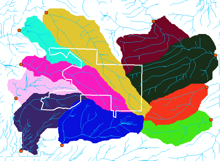
Arcata Forest drains into two main watersheds, the Mad River and Arcata Bay! Depending on the pour points you selected, you may see many more "watersheds" or fewer depending on where you placed your pour points.

Map of the watersheds

The last step is to convert this into a polygon shapefile which will be much easier to work with and will be easier on the eyes!

In the search box, enter "Raster to polygon".
At this point, we're going to be giving you fewer instructions in the labs as you're beginning to master running ArcGIS. For this tool, just make sure to uncheck the "Simplify polygons" option as we want our polygon and exactly match our raster and we can always simplify it later if desired.

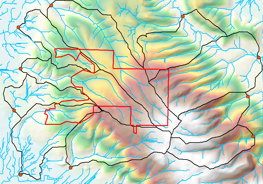
For your report, include a map of the watersheds, pour points, and streams. Use a nice hillshade but make sure to make the contract low or make it relatively transparent so it does not interfere with your key message. The one below is just to give an idea of the final map. Yours should include the required elements, labels, and look nicer!

Final map of the watersheds, streams, and pour points

Computing geometries

For our report, we need to include the number of streams, their length, and the number of watersheds, and their area. For the report, we'll be using the streams that drain at least 100 pixels (include the area of these watersheds in your report). To compute the length of the streams, add a "Length" field to the attribute table and then use "Calculate Geometry" to compute the length of each stream. Then, you can export the table to a CSV file and compute the total length of streams in MS-Excel.

Other Resources

Esri Help

Geospatial Activities