Lab 7: Working with Publicly Available Lidar in ArcGIS Pro

Introduction

Lidar point cloud datasets that can be managed, visualized, analyzed, and shared using ArcGIS. ArcGIS Pro supports lidar data provided as LAS format (industry standard) and the ESRI specific Optimized LAS (.ZLAS) format. There are a variety of tools available to process, view and edit lidar data in ArcGIS Pro. One of the most efficient ways to utilize Use lidar as a LAS dataset The LAS dataset provides fast access to large volumes of lidar and surface data without the need for data conversion or importing.

About the Data
This data is lidar points clouds data available through the USGS 3D Elevation Program through the National Map. The area of interest is Montgomery Woods State Natural Reserve in Mendocino County. The reserve originated with a nine-acre donation by Robert Orr in 1945 and has since been enlarged to 2,743 acres by purchases and donations from Save the Redwoods League. A 367.5-foot redwood at Montgomery Woods was once thought to be the tallest tree in the world. Taller trees have since been found in Humboldt Redwoods State Park and Redwoods National Park, but Montgomery Woods is still noted for its lofty giants. The lidar data was collected in 2016.

Obtaining and Extracting Lidar Point Cloud Data

 

1. Copy the data from the Z: or Google Drive to your local workstation. Make a folder for your work with the following subfolders: LAZ, LAS, Rasters. Transfer the zipped Shapefile of Montgomery Woods State Natural Reserve in Mendocino County to your data folder. Extract the LAZ files into the LAZ folder you created. Note you are missing one LAZ file (on purpose) and will have to download this file from the USGS National Map website. Keep the shapefile zipped or keep a copy of the zipped shapefile if you extract it (we will need the zipped file in the next steps).

2. Go to the National Map Download site. A variety of elevation, topographic and lidar data are available through this site including point cloud lidar data.

3. Click the upload the shapefile button and select the zipped Shapefile of Montgomery Woods State Natural Reserve (note that the boundary has been buffered by 100 ft to ensure the entire property is covered.)

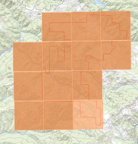
4. You should now see the outline of the reserve, zoom in so the map is focused on the area of interest. This will help ensure we select the appropriate files. Click Extent for area of interest and draw a box around the reserve polygon. This will only search for files within the bounding box.

5. Under Data select Elevation Source Data (3DEP) - Lidar > Lidar Point Cloud (LPC) then click the blue Search Products
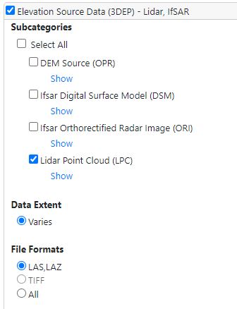
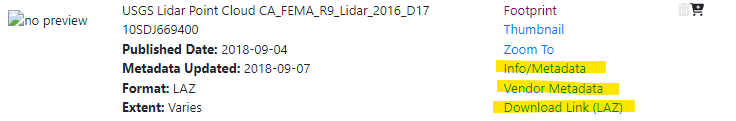
6. There are multiple tiles that cover some of the area. We want data that was all collected at the same time, so we will use the data from 2018 rather than 2022. Download the following LAZ file: USGS Lidar Point Cloud CA_FEMA_R9_Lidar_2016_D17 10SDJ669400. Download the associated metadata as well.
7. After the file has downloaded, move this LAZ file to the others in your LAZ folder. Now you have the complete dataset for the area with 13 LAZ files in your folder.

Create ArcGIS Project and Decompress LAZ Files

8. Start and sign into ArcGIS Pro. Make sure the extensions are enabled including the Spatial Analyst and 3D Analyst. Save your project as Montgomery Wood Lidar in your Lab folder.
9. In the Catalog pane add your Lab folder as a folder connection to the project. This will make it easier to find and organize our data.
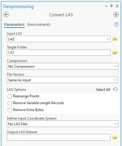
10. The first step to viewing the lidar data is to decompress the LAZ files. The compressed LAZ files will need to be converting or decompressed into the LAS format before they can be viewed or analyzed in ArcGIS. In the Geoprocessing Pane locate or search for the Convert LAS Tool (Conversion Tools > Point Cloud> Convert LAS) and launch the tool.
11. The Convert LAS tools allows the user Converts .las, .zlas, and .laz files between different LAS compression methods and file versions. In this tool you can select a single LAZ/LAS file or an entire folder to compress/decompress. To convert all LAZ files, select your "LAZ" folder as the Input LAS. This will convert all applicable files located in this folder. Select the "LAS" folder as the Target Folder. Compression should be set to No Compression (extracts or decompresses files) . Save the output LAS Dataset as MontgomeryWoods.lasd.
12. Once the tool has finished running check the LAS folder to make sure that there are 13 LAS files in the folder. The LAS Dataset should automatically be added to your map. By default you will only see the footprint of each individual LAS file.

Creating and Viewing LAS Dataset

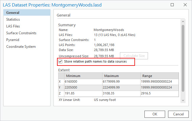
13. In the Catalog right click on the LAS files and select properties. Check the Coordinate System information.  Make note of the linear units and the Horizontal and Vertical Coordinate System. Under the General tab check the Store relative path names to data sources box.
14. Right-click on the new LAS Dataset and select Properties > LAS Files tab. After all of the files have been added you will see the file names and basic statistics for all of the LAS files.  Make note of the point spacing for all of the files and calculate the average point spacing the dataset.
15. Click on the Statistics option and click the Calculate button to produce the statistics for this LAS dataset from the LAS files you added.
16. Review and find the following information: How many different return categories are there? How many points total? You will need this information for your lab turn in.
17. Now add the shapefile showing the boundary of the reserve. By default you will only see the outline of the footprints of the LAS files that make up the dataset. There are too many points to draw. If you zoom to ~1:2,000 scale you should see the points.
18. Zoom back out so only the outlines of the LAS tiles are visible. Click on one the LAS files. The pop-up will display information for the selected file. The ability to view statistical information for LAS files referenced by the LAS dataset is essential to better understand the lidar data that you are working with. You can view general information in the pop-up, including the point count, spacing and density, as well as more detailed information on the return values and classification codes that are available for the selected file.
19. What is the average point spacing and point density of the LAS files? Use the Statistics and pop-up information to find the information
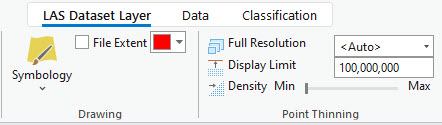
20. Zoom back into the LAS data until you can see points. Now we can check out different ways to visualize the data points in 2D. Click on the .lasd file in the contents pane to select it as the active layer. Now there will be a LAS Dataset Layer tab in the main ribbon. Click the LAS Dataset tab. This controls the appearance and how the LAS data is displayed.
21. First change the Point Thinning options. This allows some control over how many points can be rendered on the map. The density allows for more or less points. The maximum Display Limits is 100,000,000. Try increasing the display limits (if your computer is having a hard time rendering the points you may want to reduce the limit and density).
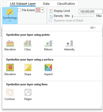
22. Check out the Symbology options. You can visualize the points by different attributes, including Elevation, Class and other attributes (vary depending on the data). You can also symbolize the layer as a surface rather than points. Try out the different symbology options.

Filtering LAS Points and Evaluating Point Density

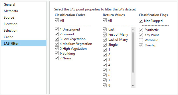
The Filters group on the LAS Dataset Layer tab set allows you to change the display of the data and display selected classes or returns. Once the filter options have been chosen, any further analysis or symbology changes will honor the selected filters. This means any statistics run or files created will be created using only the filtered points.

28. Make sure the LAS Dataset is selected in the Content pane. Then in the LAS Dataset Layer tab set, in the Filters group, check out the predefined LAS dataset filter options.
29. Click on the LAS Points button to see all of the filter options. Try filtering by specific classes and/or returns and see the different results.

Evaluate Point Spacing

We are able to get a general idea of the point spacing and density by looking at the statistics. To further look at the point density distribution we will use the LAS Point Statistics As Raster geoprocessing tool. This tool allows you to see the spatial distribution of different lidar point metrics. It does this by characterizing the points that fall into each cell of an output raster. You can choose to summarize the points in several ways:

• Pulse count
• Point count
• Predominant return count
• Maximum returns
• Predominant class
• Intensity range
• Z-range (Elevation)

30. Before starting the process, set your filters . In this case we will first evaluate the density (point or return count) for all returns, ensure filters are set accordingly. Run the LAS Point Statistics as Raster tool.
31. In tool window, select the MontgomeryWoods.lasd as the Input LAS Dataset and save the Output Raster as return-count.tif. Set the sampling value to 1 (the units for this project are in ft) this will return the number of points within each 1 sq ft pixel of the output raster. Run the tool.
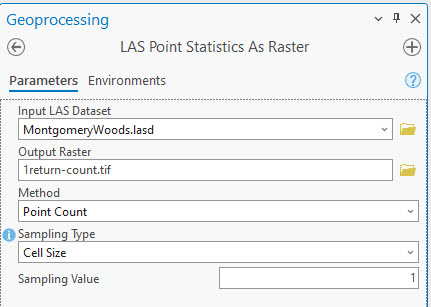
32. A new raster will be created and appear on the map once the process has finished running. This raster display the point density per square foot. Adjust the symbology to better visualize the point density data (classified or color ramp). Look at the distribution of the points, for example are there any areas with significant gaps (no data)?
33. Under the properties for the raster, look at the statistics for the point density data and copy/write-down the min/max/mean/SD stats for your worksheet.
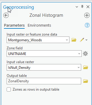
34. To determine the percentage of pixels that have no data we need to run the IsNull tool. Run the IsNull tool and select the return-count as the input. Note that the output raster will be a binary raster with 1 value=areas where there are NoData pixels and 0 everything else (has data values).
35. Run the Zonal Histogram tool to determine the count of no-data pixels within the Montgomery Woods Reserve. Use the boundary polygon as the Input Feature Zone and the layer created in the previous step as the Input Value Raster. The output table will show a count of the null or no data pixel (Label "1") and pixels with data (Label "0"). Use the pixel count information in the table to calculate the percentage of pixels with no data values.
36. Now filter the LASD data so only ground points are displayed. Rerun the LAS Point Statistics As Raster tool this time saving the file as ground-count.tif (keep all other settings the same).
37. Repeat the 32-33 for the ground statistics file. Change the symbology and look at the stats for this file.
38. When the cell size is set to 1, there are significant areas that don’t include any ground points. This suggests we should use a larger cell size to ensure there are adequate ground points. Run the tool one more time with the ground points, this time setting the sampling cell size to 3.
39. Compare the results of the different sampling cell sizes. The 3 ft sampling size should have reduced the areas without any data points. This will be the resolution we will use to create our DEMs and other surface models.

Apply a Surface Constraint

The Surface Constraints tab displays each surface constraint enforced in the LAS dataset. Surface constraints are surface features stored in either geodatabase feature classes or shapefiles. We are going to use the shapefile of the boundary of the reserve as Surface Constraint that will clip the processing results to the polygon. Note that the points won’t be clipped on the map in the LASD but should be clipped when displayed as a surface.

40. In the Catalog pane, right click on the Montgomery Woods LAS Dataset and select Properties. Click on the Surface Constraint tab.
41. Click Add and the plus button beside Surface Constraint to select the file. Find the Montgomery Woods boundary shapefile and select it. Keep height source as and select Hard Clip as surface type then click Add. Click OK to close the properties window.
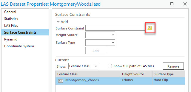
42. With the LAS dataset selected in the Content pane, select the Surface Constraints icon from the LAS Dataset Layer Appearance. Check the Surface Constraint to enable it.

Create Bare Earth Digital Elevation Model (DEM)

43. Filter the LASD data so only ground points are displayed. This will ensure only ground points are processed.
44. Now we will use the LAS Dataset to Raster tool to generate different digital surface models starting with a bare earth DEM. Either select the LAS Dataset to Raster tool from the geoprocessing menu or go to the Data tab under the main ribbon and select Export > Export to Raster.
45. In the Under Input LAS Dataset, select the LAS Dataset (.lasd). Make sure you select this from the dropdown not by clicking on the file folder, this will preserve the filter we set in the previous steps. Save the output raster as "DEM.tif” in your "Final" folder. Keep the Value Field as “Elevation” as we want to create an elevation raster.
46. Under Interpolation Type keep “Binning” selected and under Cell Assignment Type select “Average” and Natural Neighbor as the Void Fill Method. The last thing we are going to change is the Sampling Value, set this to “3”. This defines the spatial resolution of our output raster, which will be 3 feet. Then run the tool.
47. Your DEM should appear when the process is complete. This is a bare earth model showing the elevation of the ground.

Create a Digital Surface Model (DSM) that represents the Canopy and Create Canopy Height Model (CHM)

48. Now filter the LAS dataset so only the first return points are displayed. This will produce a model that represents the highest features (canopy top).
49. Use the LAS Dataset to Raster tool to generate a DSM representing the canopy. Keep the same inputs as before except change the Cell Assignment Type to “Maximum” keep the sampling cell size the same (3) and save the file as dsm.tif, then run the tool.



With both the DEM and DSM generated from the lidar data it is possible to estimate the canopy height above the ground. The DSM is essentially the height of the canopy above sea level. We want to create a raster that solely represents the height of the canopy above ground. This can be done by simply subtracting the DEM from the DSM, which produces a canopy height model (CHM) or what can also be referred to as digital height model (DHM)

50. We will create a canopy height raster by subtracting the two rasters. Use the Minus geoprocessing tool (you could also use the raster calculator to accomplish this).
51. In the Minus tool, For Input Raster 1 select the canopy surface model "DSM.tif" and for Input Raster 2 select the DEM "DEM.tif", so DSM-DEM = CHM (Canopy Height Model). Save the output raster in your raster folder as “CHM.tif” and click OK.
52. You will now see the canopy height raster in your viewer. The values in this raster represent the height of the vegetation above ground (in feet in this example). We will need to do a little further clean up on the data. Note that we have negative canopy height (which should be set to 0) and extremely large values due to outliers in the first returns. Some of these points in the LAS files should be classified as noise, but many of the very tall trees have also been classified in the same class. There are a couple of approaches to dealing with classification issues:
    1. Use the the LAS Dataset tools to manually re-classify some of the points if needed. See Interactively edit LAS class codes—ArcGIS Pro for more information. This is a good approach if there are specific features or only a few easily visible points that need to be re-classified.
    2. Use the Re-Assign Classification and Classify Noise tools to re-classify the points.
    3. Use the Conditional (Con) tool to replace the values outside of the expected range.

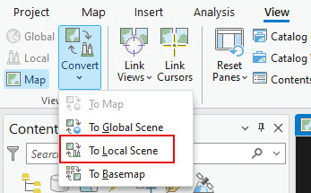
Converting a 2D Scene to a 3D Scene

53. Before we decide how to clean up the results, let's view the data in 3D. Remove all of the point statistics related files.  Keep the LASD and DEM, DSM, CHM files in your map.
54. Click View from the main ribbon and select Convert to Local Scene.  This will convert the current map to a 3D enabled scene.
55. Play around with the data and navigation in the 3D Scene. Try changing the filters to only show specific classes or returns.
56. The Classification tab allows you to interactively change the classification conducted on the LAS files in a LAS dataset in a map or scene. You can interactively change the class codes and classification flags that are currently set on the selected points. This can be useful when trying to reclassify a small number of points.

When you modify the classification codes in LAS files on disk, the changes you make are permanent. If you are conducting trial scenarios or do not want changes to be permanent, work with a copy of the LAS files and not the original data

Re-Assign Classes and Classify Noise

57. In either the 2D or 3D Map scene click on the LASD dataset and select the Re-Assign Classification tool under the Automated Classification button. This tool allows the user to re-assign specific classes.
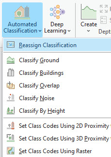
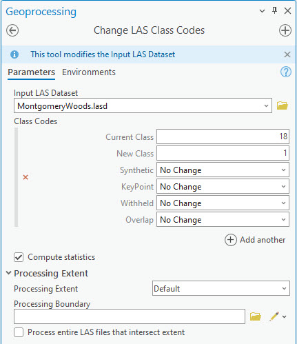
58. In the Change LAS Class Codes tool select the Montgomery Woods LASD and change the current class of 18 (High Noise class) and set the New Class to 1 (unassigned) then run the tool. This will convert all of the points classified as High Noise to the Unassigned class.
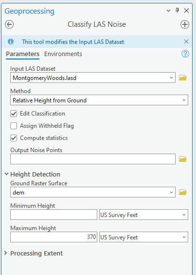
59. Now all of the points that were formerly classified as High Noise have been re-classified to the unassigned category. Now we will run Classify LAS Noise tool.
60. Select the Montgomery Woods LASD as the Input and Relative Height from Ground as the Method. Select the DEM as the Ground and 370 feet as the Maximum Height. The run the tool, it may take awhile, but when it is finished points higher that 370ft (above ground) will be classified as noise. Notice that the points corresponding to tops of the tall trees are now unassigned class.

Classify LAS by Height

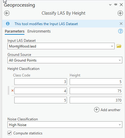
The Classify LAS By Height tool reclassifies LAS points with class code values of 0 (never classified) or 1 (unassigned) based on their height from the ground surface created using LAS points with class code values of 2 (ground). Classifying points using height gradients from the ground surface can provide a useful way to visualize and filter the point cloud which can also aid the process of conducting more refined interactive classification. The tool defaults to classifying class codes 3, 4, and 5, which represent low, medium and high vegetation in the ASPRS specification for the LAS format, but the height settings may be changed based on project location and objective. We will use this tool to re-classify the

61. Run the Classify LAS by Height tool either through the Geoprocessing pane or from the Automated Classification tab under LAS Dataset in the main toolbar ribbon. Note this tool edits the original LAS file by changing the classification of specified points.
62. In the tool select the Montgomery Woods LAS dataset as the Input and All Ground Points for Ground Source. Set the Height for the class codes as follows: Class 3 (Low Vegetation) : 5, Class 4 (Med Vegetation) : 75 and Class 5 (High Vegetation) : 370. Note that the Z units (elevation) for this data are in feet. This means all non-ground points between 0 and 5 ft will be classified as “Low Vegetation”, between 5-75 ft Medium and 75-370ft High vegetation. Set the Noise Classification to High Noise and check the Compute Statistics box, then run the tool. It may take a few minutes.
63. Once the process is complete the LAS dataset should update including the statistics. Review the statistics for the LAS dataset and change the symbology to classified to see the effects.

Create the DSM and CHM excluding the Noise Classes

64. Go back to your 2D map. We are going to rerun the DSM and CHM, this time filtering out the points that are marked as Noise (both Noise and High Noise), but keeping all other settings the same. Re run steps to create the DSM and CHM with the noise points excluded. Keep the same settings but save the files as DSM_NoNoise.tif or something similar.
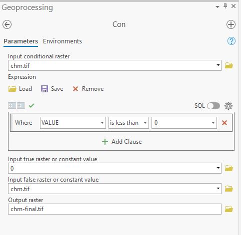
65. Depending on the data, you may still may encounter negative CHM values. We will remove any negative values (noise) using the Con geoprocessing tool to recalculate any negative values to a value of zero. In the geoprocessing pane select the Con tool by searching for it or by locating it under Spatial Analysis Tools→ Conditional → Con.
66. In the Con tool window, select the CHM files has the Input conditional raster. In the Expression box enter Value < 0, this will apply the tool only to pixels where the canopy height value is less than 0. Type "0" in the Input true raster or constant value. This will replace any values less than 0 (negative values) with 0. In the next box, Input false raster or constant value select the CHM file. This will use the existing CHM values for all areas where the values are greater or equal to 0. Save the file as CHM-final.tif in the Finals folder and hit OK.
67. Review the statistics (min/mean/max) for the final DEM and CHM data. Create a histogram of the final canopy height data using the chart tool.
68. Finish filling out the worksheet and back-up your data for next week! To reduce the file size you can remove the LAZ folder.