Lab 7 - Part 2: More Lidar in ArcGIS Pro

Introduction

This exercise is a continuation of Lab 7 Part 1 - Working with Publicly Available Lidar in ArcGIS Pro. The clipped lidar dataset of Goukdi’n- Jacoby Creek Forest that was generated in the previous exercise will be used. This lab exercise will focus on creating and visualizing the lidar derived data products and extracting further information from the lidar data.

About the Data
This data is lidar points clouds data available through the USGS 3D Elevation Program through the National Map. The area of interest is Cal Poly Humboldt owned Goukdi’n- Jacoby Creek Forest.

View Data in 3D

1. Copy your data from the previous Lab from Z: or Google Drive to your local workstation. Open ArcGIS Pro and open up the previous map project with the Clipped JCF lidar LAS Dataset. At this point that data should be extracted to the polygon boundary and vegetation points classified
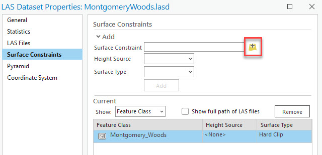
2. Apply the Forest Boundary polygon as a Surface Constraint to the Clipped LAS Dataset. In the Catalog pane, right click on the Clipped JCF LAS Dataset and select Properties. Click on the Surface Constraint tab.
3. Click Add and the plus button beside Surface Constraint to select the file. Find the JCF boundary shapefile and select it. Keep height source blank and select Hard Clip as surface type then click Add. Click OK to close the properties window.
4. With the LAS dataset selected in the Content pane, select the Surface Constraints icon from the LAS Dataset Layer Appearance. In the Layer Properties window, check the Surface Constraint to enable it.

Create Bare Earth Digital Elevation Model (DEM)

5. Filter the LASD data so only ground points are displayed. This will ensure only ground points are processed when the DEM is created.
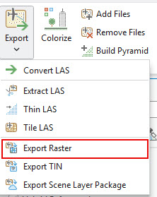
6. Now we will use the LAS Dataset to Raster tool to generate different digital surface models starting with a bare earth DEM. Either select the LAS Dataset to Raster tool from the geoprocessing menu or go to the Data tab under the main ribbon and select Export > Export Raster.
7. In the Under Input LAS Dataset, select the LAS Dataset (.lasd). Make sure you select this from the dropdown not by clicking on the file folder, this will preserve the filter we set in the previous steps. Save the output raster as "DEM.tif” in your "Raster" folder. Keep the Value Field as “Elevation” as we want to create an elevation raster.
8. Under Interpolation Type keep “Binning” selected and under Cell Assignment Type select “Average” and Natural Neighbor as the Void Fill Method. The last thing we are going to change is the Sampling Value, set this to “1”. This defines the spatial resolution of our output raster, which will be 1 meter. Then run the tool.
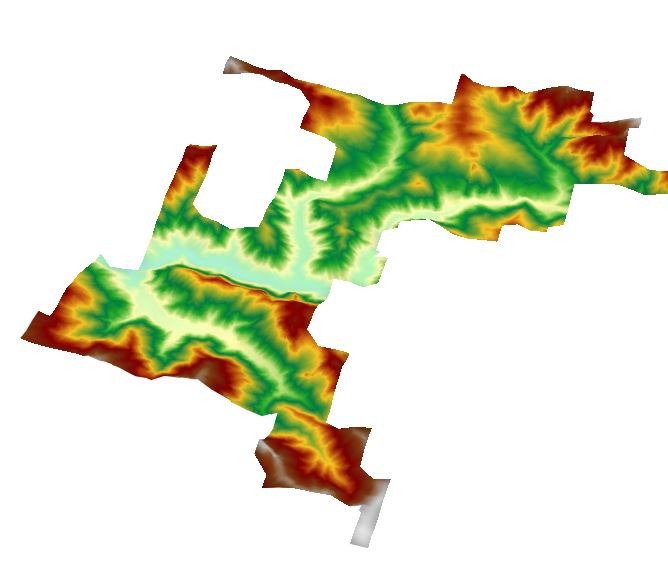
9. Your DEM should appear when the process is complete. This is a bare earth model showing the elevation of the ground.

Create a Digital Surface Model (DSM) that represents the Canopy and Create Canopy Height Model (CHM)

10. Now filter the LAS dataset so only the first return points are displayed. This will produce a model that represents the highest features (canopy top).
11. Use the LAS Dataset to Raster tool to generate a DSM representing the canopy. Keep the same inputs as before except change the Cell Assignment Type to “Maximum” keep the sampling cell size the same (1) and save the file as dsm.tif, then run the tool. this will use the highest recorded point elevation as the cell value.



With both the DEM and DSM generated from the lidar data it is possible to estimate the canopy height above the ground. The DSM is essentially the height of the canopy above sea level. We want to create a raster that solely represents the height of the canopy above ground. This can be done by simply subtracting the DEM from the DSM, which produces a canopy height model (CHM) or what can also be referred to as digital height model (DHM)

12. We will create a canopy height raster by subtracting the two surface rasters (DSM-DEM). Open the Minus geoprocessing tool (you could also use the raster calculator to accomplish this).
13. In the Minus tool, For Input Raster 1 select the canopy surface model "DSM.tif" and for Input Raster 2 select the DEM "DEM.tif", so DSM-DEM = CHM (Canopy Height Model). Save the output raster in your raster folder as “CHM.tif” and click OK.
14. You will now see the canopy height raster in your viewer. The cell values in this raster represent the height of the vegetation above ground (in meters in this example).

Converting a 2D Scene to a 3D Scene

15. Before we decide how to clean up the results, let's view the data in 3D. Keep the LASD and DEM, DSM, CHM files in your map. You may remove any other layers previously created.
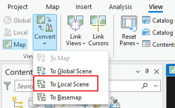
16. Click View from the main ribbon and select Convert to Local Scene.  This will convert the current map to a 3D enabled scene.
17. Play around with the data and navigation in the 3D Scene. Try changing the filters on the LAS Dataset to only show specific classes or returns. Use the center wheel to control navigation, including the zoom level and the view angle.
18. Right-click on the Ground element under the Elevation Surfaces group at the bottom of the Content Pane and select Add Elevation Source. Select the DEM, CHM & DSM from the project folder then click OK. Remove the default "WorldElevation3D/Terrain3D" layer.
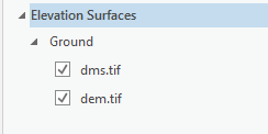
19. Any layer added to the 2D layers group will be draped over the elevation surface. Note that the DEM is the bare ground elevation and terrain, while the DSM includes the elevation of the above ground vegetation in addition to the ground. Turn the the elevation surface layers on and off to see the differences between the options.
20. Now add the Imagery Basemap to your 3D map. This will display a recent satellite or aerial image or the area. Try turning on and off the different layers and experimenting with the display options. Turn on the various height model rasters and see how they look in the 3D scene. For more information on navigating in scenes and linking scenes check out the Navigate maps and scenes in ArcGIS Pro video. Either stay in the 3D scene or return to the 2D scene for the next steps.

Calculate Point Density for Ground and Aboveground Points

The most effective way to determine the canopy density is to divide the study area into small, equal-sized units through rasterization. In each raster cell, you compare the number of above-ground points to the total number of points to estimate the density or cover percentage. The process will create a raster where the values range from 0 to 1, with 0 representing no canopy cover and 1 representing total or 100% cover.

21. Ensure the points in the LAS Dataset are filtered to only show the ground points.

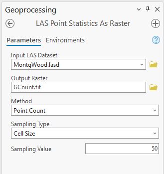
22. Use the LAS Point Statistics As Raster tool to calculate the ground point count for each cell, setting the sampling value at 15 (15 meters).
    Save the file as groundcount or gcount, you may either save as a TIF or as a raster in the default geodatabase.
23. Now filter the points so only the medium and high vegetation classes are selected. This will exclude lower ground vegetation and ground points from the canopy cover analysis.
24. Repeat the for the aboveground points, keeping the cell size the same. When you are done you will have two files showing the pointy density for the ground and aboveground points

Create Model in ArcGIS Pro to calculate the Canopy Density (cover %)

To properly calculate the percent canopy cover, we need to convert any resulting NoData cells to 0 so that subsequent operations treat a cell with no points as 0. This is accomplished using the IsNull geoprocessing tool followed by the Con geoprocessing tool. An easy way to do this is to use the ArcGIS Pro ModelBuilder. The ModelBuilder is used to create, edit, and manage geoprocessing models that automate those tools. Models are workflows that string together sequences of geoprocessing tools, feeding the output of one tool into another tool as input. ModelBuilder can also be considered a visual programming language for building workflows and is very similar to the ENVI Modeler environment.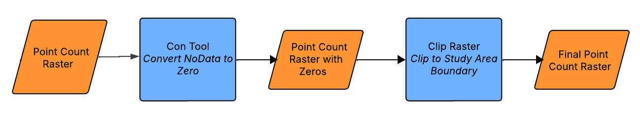

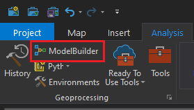
25. On the Analysis tab, in the Geoprocessing group, click ModelBuilder. This will launch the ModelBuilder window.
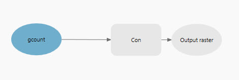
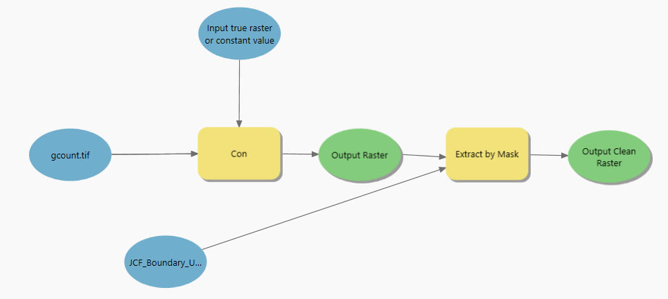
26. To add data to your model, drag layers from the map Contents and datasets from the Project into the model. The layers and datasets are added to the model and displayed as input data variables. Add the ground point density (count) ‘gcount’ file to the model by dragging it into the model window.
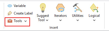
27. To add a geoprocessing tool to your model, ensure the model view is active, then start typing to search for under Tools in the ModelBuilder pane and double-click a tool to add it to the model. Alternatively, you can drag a geoprocessing tool into the model from the Geoprocessing pane or Catalog pane. Add the Con tool to the model.
28. Connect the point density raster to the Con tool, selecting it as the Input conditional raster.
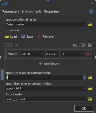
29. Double click on the Con tool. Under the Expression parameters, set the expression to select vales that are null: Value: Is Null. Set the Input true value to 0 and the Input False Raster as the Model Variable "gcount". This means that when there are null pixels they will be converted to 0s and if not (false), they will retain their original value (from the ground point count file). Don't worry about naming the output raster, there is still another step in the model process. click OK to close the Parameter window.
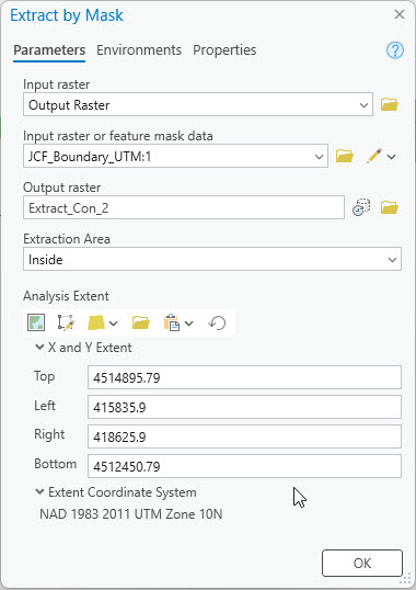
30. Now add the Extract by Mask tool to the model. Connect the output of the Con tool to the Extract by Mask, setting this as the Input Raster for the tool.
31. Open the Extract by Mask tool settings in the model. Set the Feature Mask as the boundary shapefile and st the Extraction Area to Inside, this will clip or remove areas outside the defined polygon boundary. Click OK to close the window.
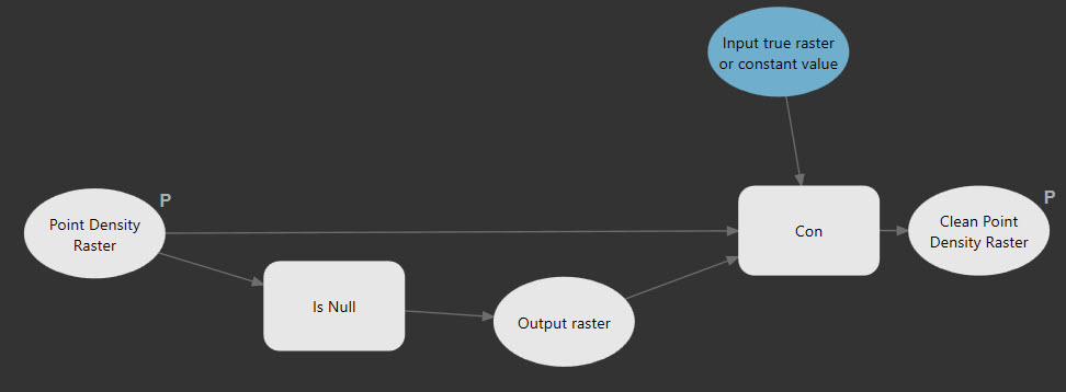
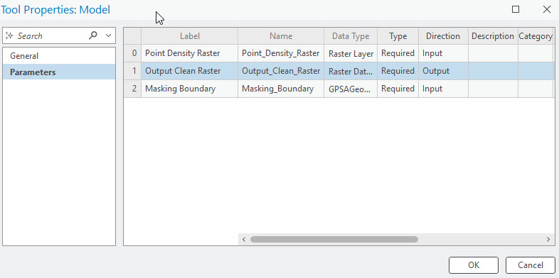
32. The model should be in color now, indicating it could be run now, but it wouldn't allow us to specify any alternative files or how to save the files. The last step is the Parametrize the model and remove some of the default files selected for processing. This makes the selected variables a user-configurable input when the model is run as a geoprocessing tool.
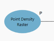
33. Add parameter to the Initial input (point count raster) by right clicking and selecting Parameter.  This will add a parameter input window when you run this model as a geoprocessing tool. Right click again and rename the initial input to a more generic title like Point Density Raster.
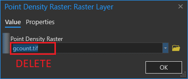
34. Even though we “parameterized" the input and output rasters, the model still defaults to using the ground count dataset. This isn't going to make much sense if you share your model or toolbox with other people or use the tool on different datasets. To remove the default dataset, double-click the Point Density input element and delete the path, then click OK. Some of the elements in your model may turn gray. This signifies that a value must be provided before the model can successfully run.
35. Repeat the above two steps to Parameterize the extraction boundary by right clicking on the JCF Boundary Polygon input and selecting Parameter. Delete the existing data path and re-name the variable Extracting Boundary or something similar.
36. Right click on the final green output file and select Parameter. This will allow you to select the file name and location that the final file will be saved to. Rename the node to a more generic name like Clean Point Density Raster.
37. Save your model! Save in your project toolbox as Clean Up Point Density (or something similar).
38. Roll over each of the elements and check to see if there are any paths or file names listed for the tools. If so, open and delete the path/filename. To adjust the order that the parameters appear in the tool, go to Model > Properties. In this window you can move the order of the parameter. Save your modelwhen you are done!
39. Run your model but run it from the geoprocessing tools or from the toolbox. An input dialog will open and you can specify the files for the input and where/how to save the output file. Run the tool using the ground density raster and again using the aboveground density raster and save the output files (clean ground and abg points) in your raster folder. Note that you will need to upload your toolbox with your model as one of the turn-ins for this lab.

Calculate Cover Model

To calculate the cover or canopy density we need to add the aboveground and bare earth rasters together to get a total count per cell using the Plus geoprocessing tool to get the total points (ground + vegetation above 6ft). Note that all the count rasters you've made so far are long data types. You need one raster to be floating point to get floating-point output from the Divide geoprocessing tool that you will use. To generate a float raster, use the output raster from the Plus geoprocessing tool as input to the Float geoprocessing tool. Then finally we will use the Divide geoprocessing tool to compare the aboveground count raster and the floating-point total count raster. This gives you the ratio from 0.0 to 1.0, where 0.0 represents no canopy and 1.0 very dense canopy.

40. Add the “LidarTool.txb” (provided with in the lab data folder) toolbox to your project by selecting Toolbox under the Insert tab in the main tool ribbon.
41. In the catalog pane locate the toolbox. There should be one tool in the toolbox entitled Canopy Cover. Right click on the Canopy Cover model and select open.
42. This model has been created to simplify the process of calculating the cover. Notice that all the various nodes are gray instead of colored. This means that the data has not been specified in the model and the user will be prompted to select appropriate input files and where/how to save the output files when the tool is run.
43. Run the Canopy Cover tool through the geoprocessing pane or Catalog pane. Select the appropriate ground and above ground rasters for the inputs and save the file as canopy.tif in your rasters folder.
44. When the process is complete you should have a file in your map that represents the canopy density, with 1 being 100% cover and 0 indicating no cover.

Use the CHM to Locate the Tallest Trees

45. Use the Raster Calculator to locate the trees with canopies height greater than 70m. Use your CHM layer in the raster calculator expression. The result should be a binary raster, with ‘1‘ values indicating canopy greater than the set level.
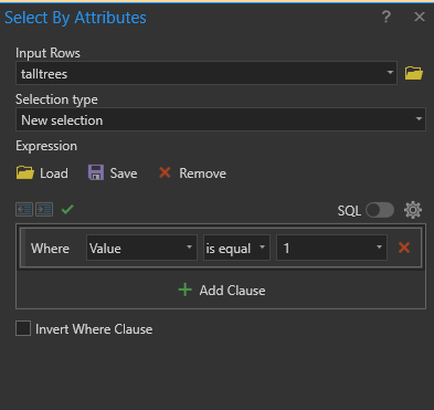
46. Open the Attribute Table for the “talltrees” layer you just created and select the row containing the “1” values.  The pixels with 1 values should now be highlighted light blue on the map. You could also use the Select by Attribute function to select the pixels where the value field is equal to 1.
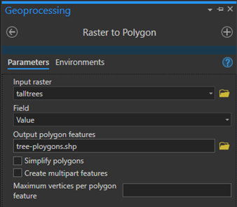
47. Take a look at the results and compare the pixels to the canopy height model. Notice that the pixels are grouped together and several pixels represent an individual tree. Now we will create polygons from these selected pixels so each group of pixels is grouped together into a single polygon. Run the Raster to Polygon tool to accomplish this.  Select the “talltrees” as the input file from the drop down.  Field should be set to Value and save the polygon as tree-polygon.shp and run the tool.
48. Now we have a shapefile with polygons showing the locations of the tallest tree canopies.  For visualization and mapping purposes we will also create a point shapefile showing the locations of the tallest trees. To do this run the Feature To Point  tool. Select the tree polygons as the input feature and name the outpost feature class as tree-points.shp and run the tool.
49. We now have the locations of the tallest trees. Review your final locations and cleaned-up tree-points layer removing any erroneous or duplicate points. If you make any edits you will need to save your edits (under the Edit tab in the main toolbar) before completing the last steps.
50. Create a slope layer from the DEM file using the Slope geoprocessing tool or using the Raster Function
51. The Extract Multi Values to Points tool extracts pixel values at point feature location from one or more rasters and records the values to the attribute table of the point feature class. Under input rasters add the canopy height, elevation (dem) and slope value. Then run the tool.
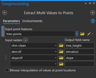
52. You should now have a point feature layer that includes the elevation, height and slope attributes of the locations of the tallest trees. Open the attribute table for the point layer.
53. Now we will add the coordinates of the points to the attribute table. Run the Calculate Geometry Attributes geoprocessing tool.  Select the tree-points layer as the input feature.  We will add two new fields for the latitude and longitude (see below).  The latitude is the y coordinate and longitude the x-coordinate.  Select Decimal Degrees as the coordinate format and Current Map for the coordinate system and run the tool.  Now the coordinates have been added to the attribute table. Copy the information from the attribution into a spreadsheet.

Find the Highest and Lowest Ground Elevation

54. Using some of the same above methodology find the lowest and highest ground elevation areas in the forest and create a point feature that shows the locations. Consider using the Raster to Point Conversion tool rather than the Raster to Polygon to simplify the process.

Create Hillshades and Maps

55. Create hillshades for the CHM, DEM and DSM. You can either use the Raster Functions tool to generate a hillshade on the fly (no file is saved) or use the Hillshade geoprocessing tool to save a hillshade for each layer. These will be used to create the final maps.

56. Create three maps, one showing the canopy cover percent, one with the canopy height model and one showing the elevation. All maps should use the appropriate hillshades to provide relief shading, the maps may be 2D or 3D. The elevation map should display the bare earth terrain, elevation color ramp and the low and high elevation location. For the canopy height map use either the DMS or CHM hillshade, the canopy height in color and optionally the locations of the tallest trees.

Turn In

• Map with the Canopy cover model and appropriate hillshade.
• Map with Elevation and bare earth hillshade displaying the low and high elevation locations
• Map with final cleaned up Canopy Height Model and appropriate hillshade (with or without tall tree locations)
• Upload the toolbox with your parameterized model that cleans up the point density rasters

• Answer the following two questions:

  1. How many trees did you locate that are taller than 70 meters?
  2. Where do the tallest trees appear to be located in terms of topography?
• Cleaned-up, formatted version of the attribute table showing the object id, tree height, slope, elevation and location coordinates (lat/long).