Lab 2- Part 2: Image Visualization in ArcGIS Pro

Introduction

In this lab we will cover techniques for visualizing data and creating maps with remotely sensed data in ENVI and ArcGIS Pro.

Learning Outcomes

• Download SRTM DEMs in ENVI
• Importing satellite imagery and data into ArcGIS Pro
• Evaluating Image Statistics and histograms
• Visualizing data in ArcGIS Pro
• Creating hillshades and other surface derived layer
• Creating maps from remotely sensed data

About the Data
The primary data for this lab is Landsat Collection 2 Level-1 data that has been calibrated and corrected to Surface Reflectance in the previous lab exercise. From this data a Spectral Index layer was created which will also be used in this lab exercise.

Adding Custom Tasks in ENVI

You will begin by copying over your Lab 2 Final data folder from the previous lab. ENVI Custom Tasks can be created using the ENVI Modeler. These tasks can be saved and added to the Toolbox in ENVI. When ENVI is launched it will automatically scan specific folders for custom tasks

1. You will begin by copying over your Lab 2 Final data folder (from the previous lab) to the desktop. You will need the masked surface reflectance and spectral index data (e.g. NDVI or NBR) for this lab.
2. From the shared drive download the .task file and copy the file to the ENVI custom code file folder under your user profile on the computer: C:\Users\username\.idl\envi\custom_codex_x Start
3. Start ENVI and open your SR_Masked.dat Landsat image. This file was generated in the previous lab exercise and represents the surface reflectance data with the no data areas masked. Open your masked spectral index file also generated in the previous lab exercise.
4. Navigate to the Toolbox >Task Processing >Run Task. This will bring up the list of ENVI Tasks and Custom Tasks that can be run. Check to make sure the task "Hi/Low Clip" is on the list. This is the custom task added in the previous steps.
5. Looks at the statistics for your spectral index layer. Note if there are any values outside the expected range. For example NDVI values greater than 1 or less than -1. Clip or Mask Values Outside Expected Range using one of the two methods:
   1. Mask: Use the ROI Threshold Tool to find and isolate values outside the expected range and apply a mask to "hide" or remove these values.
   2. Hi Low Clip Task: Use the Hi Low Clip Task to set to set values outside the set range, e.g. set values less than -1 to -1.

   Download SRTM Elevation Data in ENVI

   6. Now we will download a Digital Elevation Model of the region to use later when creating maps. There is a built in DEM downloader in ENVI that downloads data from the SRTM (see more below).In ENVI, select File > Open World Data > Download Digital Elevation Model from the ENVI menu bar.

      About the Tool and Data
      Use this tool to download Shuttle Radar Topography Mission (SRTM) raster Digital Elevation Model (DEM) data. SRTM raster DEM data is available from https://srtm.csi.cgiar.org/. The SRTM data available through this download option is global, 90 m spatial resolution. The Download SRTM Raster DEM dialog appears. Follow the steps below to define an area of interest, buffer distance, and output coordinate system for the download.

      
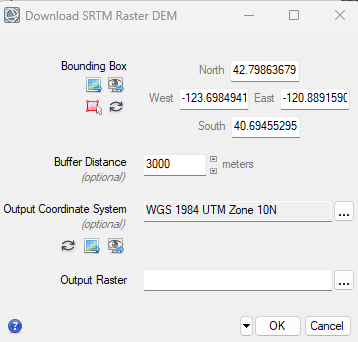
   7. Set the Bounding Box as the Surface Reflectance data. This will download a DEM that covers the entire region of the Landsat image. You can also specify other extents manually or using current view. Set the Output Coordinate System to also be the same as the Surface Reflectance data. This means the data will automatically be re-projected to whatever coordinate system you select.
   8. Save the output raster as DEM.dat in your finals folder and click OK.
   9. After downloading and processing the DEM will appear in the window. It should cover the extent of the Landsat image.

   Chip to PowerPoint Options

   10. Display the Landsat image area you want to chip in one view or multiple views. You can use the Zoom, Pan, Rotate, and enhancement tools to customize the display. Layers can also include images, vectors, regions of interest (ROIs), etc.
   11. From the menu bar, select File > Chip View To > PowerPoint. Or click the Chip To PowerPoint button in the toolbar. The Chip to PowerPoint dialog appears.
   12. Select an option from the Target Presentation drop-down list: Choose (Start a new presentation) to chip the views to a new PowerPoint presentation. If you already have a PowerPoint presentation open, choose one of them as the target.
   13. Select a predefined slide template from the Template drop-down list, then click the Configure Template button. See Chip ENVI Views to PowerPoint for more information about the templates and configurations.
   14. Click the Chip button. The views are chipped to a new slide in the selected presentation. Try out several different templates, you can try different templates and they will be added to the existing PowerPoint presentation. Decide on one slide and edit the slide as approriate. Save the slide as a JPG using the Save As function in PowerPoint.
   15. Make sure that all of you files are saved in your finals folder then you may close ENVI.

   Visualizing Raster Data in ArcGIS Pro

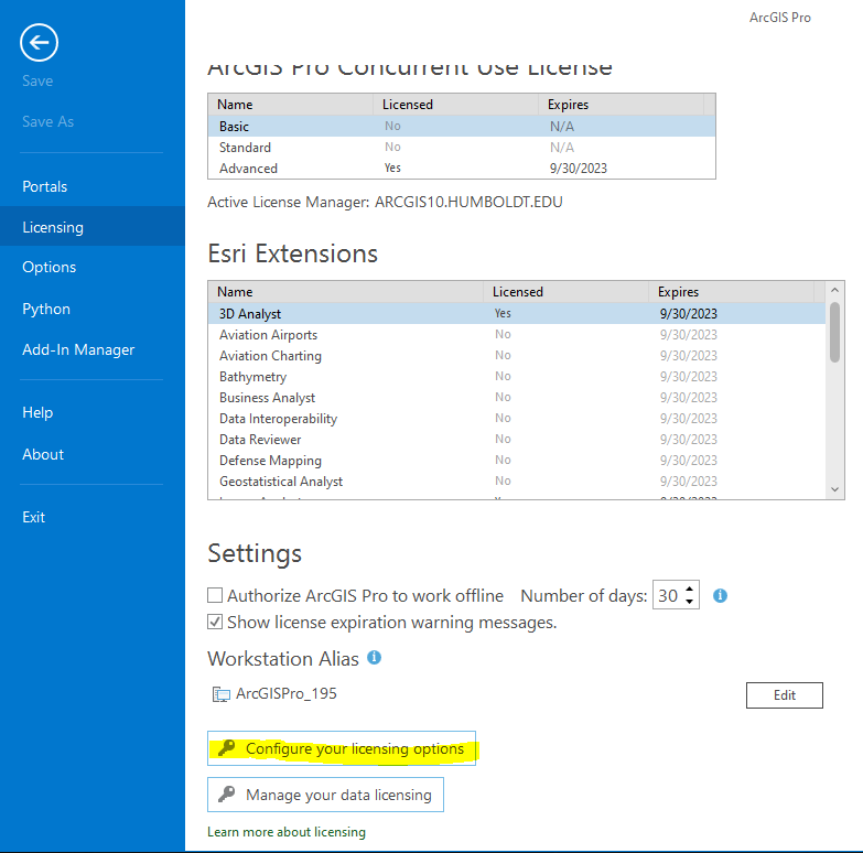
   16. Launch ArcGIS Pro and then Go to Settings > Licensing > Configure your licensing options. Check the Spatial Analyst and Image Analyst to make sure they are licensed and enabled. You may want to enable other extensions at this time as well.
   17. Open a new blank Map template, call the project Lab 2 Maps and save it to your final folder. A new project and map template are generated.
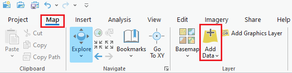
   18. Now we will add data to our map. Go to Map tab > Add Data and located the image SR_masked.dat Landsat satellite image from your lab data from the previous lab and open the image (click once to open the color multispectral imagery, double clicking allows you to open individual band). If prompted say yes to Calculating Statistics and Pyramids for the file.
   19. There are specific rendering options available for raster files in the Raster Layer tab. Explore the difference Stretch Types and their effect on the imagery. Also try out Resampling Type options to see how they alter the image.
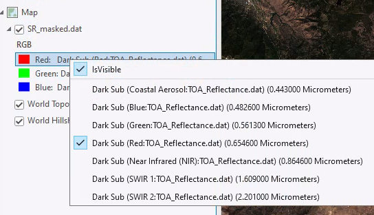
   20. You can change the band combinations to any false color composite. Right click on the layer in the table of contents and you can select which band should be displayed in which color (Red, Green, Blue). You can also set and save custom band combinations from the Band Combinations window.
   21. There are also a few more image enhancement tools that change the look of imagery. You can adjust the Contrast, Brightness and gamma. You can also adjust the rotation to change from the default of North is up when applicable.

   Visualizing Spectral Indices

   22. Now add the your spectral index layer and DEM.dat layers that you created in ENVI to your map.
   23. Change the symbology of the spectral index layer. Try out different color ramps and symbologies. Try changing the symbology to the classified option and experiment with different colors and classification schemes.
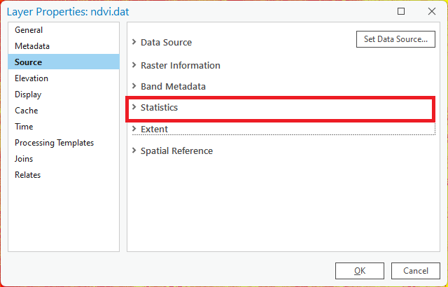
   24. Now we will investigate the statistics of the spectral index dataset. Right click on the file and select properties. In the Layer Properties window select the Source tab. This contains information about the raster, including the resolution, coordinate system and summary statistics. Click on statistics and note the mean, min, max and standard deviation of the data.
   25. Now we will view a histogram of the spectral index data. Under the Raster Data tab go to Create Chart > Histogram. The Histogram tool appears. Select the Normalized Difference Vegetation Index as the number variable.
   26. Increase the number of bins, experiment different options. Check the boxes to add the Mean and Standard Deviation to the histogram, then export the graph bu selecting Export >Export as a Graphic and saving the image in your finals folder.

   Raster Functions

   Raster functions are operations that apply processing directly to the pixels of imagery and raster datasets, as opposed to geoprocessing tools, which write out a new raster to disk. Calculations are applied to the pixels of the original data as the raster is displayed, so only pixels that are visible on your screen are processed. These tools are a great way to quickly preview an operation or to create layers for visualization. If you need to save the file or use it in future analyses the geoprocessing tools are more appropriate.

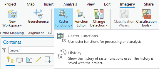
   27. Under the Imagery Tab navigate to the Raster Functions button and click on the Raster Functions. This will launch the Raster Functions pane on the side. There are many different functions to choose from.
   28. Navigate to the Surface functions in the Raster Functions tool pane. Select the Hillshade option.
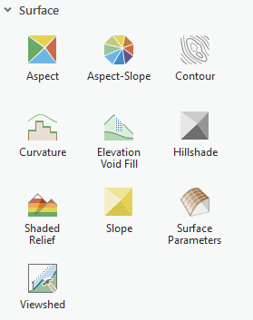
   29. Create a hillshade using the DEM as the input file (you can keep all of the default settings).
   30. Now create contours using the DEM as the input file. Now you have a few topographic layers that can be used to create maps and better visualize your data.
   31. Rearrange your layers so that the Landsat image is on top of the hillshade (you may choose to leave the contours on or off, your choice). Adjust the settings using the transparency and other enhancements to create a visually appealing satellite image where the topography is visible.

   Creating Maps

   32. Zoom in on an area of interest to focus on for your map (can be anywhere!). After zooming in go the the Map tab > Bookmarks and click New Bookmark. A bookmark is a navigation shortcut to a position on a map. Name your bookmark.
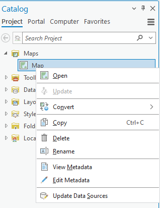
   33. Create a copy of your map by going to the Catalog Pane and right clicking on your map and selecting Copy. Paste the map in the Maps folder in the Catalog pane. Repeat the process one more time so you have three maps in your folder. Re-name the maps something like "Landsat", "Spectral index" and "Topographic". You will have three separate maps when you are done. Add the maps to your project by double clicking on them in the Catalog.
   34. In each of your maps layer the applicable data layer over the hillshade and adjust to visualization settings. One map should have the satellite imagery as the focus, another with the spectral index results and a final map with the elevation (or other topographic features) and hillshade and/or contours. All maps should utilize the hillshade to provide topographic relief.
   35. Now we will prepare the map layout, we will create one page with all three of our maps. From the Insert tab select → New Layout to add a layout to your project. Select a Landscape Letter 8.5" x 11" paper size and press OK.
   36. To add a map frame to your layout, click the Map Frame button on the ribbon. From the drop-down, Under the Landsat map select your saved Bookmark as the extent then click on the empty map page. You will now see a rectangle with the default map.
   37. Repeat this process to add the remaining two map frames. You should have three map frames on your layout, one with satellite imagery, one with NDIV and one with topography. Adjust the size of the frames and paper as you see fit. To remove the service credits remove the basemap layers from your map. You may need to switch between the layout and map views for the map to update.
   38. Now add the appropriate cartographic element, including Titles, Labels, Scale bars and North arrow. These can all be found under the “Insert” menu in the Layout View. Below is an example, your map should have different years. Also include the data sources and map author.
   39. When you are happy with your map export it to a PDF or JPG. Click on the Share tab from the main menu and select “Export Layout”. Select PDF or JPG as the type and make sure the resolution is set at 300dpi and save it in your “Finals" folder.

    

   Turn In - Maps and Histogram

   A Word document with:

   • Maps with three data frames showing (the same extent and scale ) the satellite imagery, spectral index results and a topographic map of your choosing.
   • Spectral index histogram and statistics