Lab 2: Image Processing Techniques and Introduction to ENVI Modeler
Introduction
In this lab we will cover the ENVI processing techniques for radiometric calibration, atmospheric correction and metadata updates. This lab also include an introduction to ENVI Modeler. The ENVI Modeler is a visual programming tool that enables you to create custom task-based workflows within ENVI. The user interface is designed to help users build workflows without any knowledge of ENVI programming. You can easily create custom workflows and batch-process data with the ENVI Modeler.
Learning Outcomes
- Extracting and Viewing Level-1 and Level-2 Landsat Data reflectance data.
- Perform Radiometric Calibration in ENVI
- Conducting atmospheric correction (dark object subtraction)
- Reviewing Image Statistics and updating Metadata
- Creating Customized Workflows Using ENVI Modeler
- Comparing Data Values in ENVI
- Creating Workflow Diagrams
About the Data
The primary data is this lab is Landsat Collection 2 Level-1, Landsat Collection 2 Level-2 Surface Reflectance data will be viewed for comparison.
The specific data used in the lab is a Landsat 9 image of the south central Oregon acquired May 2nd 2025.
Accessing and Reviewing Landsat Level-1 Data in ENVI
You will begin by creating a folder structure or "workspace" that will keep your files organized and prevent any confusion as you work with multiple datasets in the future. It is important to have the files you are working with on a local drive (C: in our case). Many processes in ENVI and ArcGIS do not work well or at all when data is stored in the cloud (i.e. Google Drive G: Drive) or on portable storage devices. Back up your data when you are done!
- Create a new folder on the desktop or documents folder for your lab data (recommended naming convention of the folder “GSP326_Lab_#”). Create three subfolders: original files, working and final.
When you are done, you will want to back up your final work onto a USB drive, or cloud based storage like Google Drive or the Course Share Z: Drive. The hard drives (including the desktop) on the lab computers will be deleted every 24 hours. Be sure to always save and backup your work!
- Download the Lab 2 data files from the shared Google Drive folder or the class share network drive (Z:). The data consists of two Landsat "tarball" files (.tar). Extract the two files into your original data folder, note that each of the files should be extracted into separate folders. When the process is finished you should have two folders that each contain Landsat data files, one is Level-1 data while the other is Level-2 data.. Open ENVI (ENVI 6.2).
- We will start by viewing and working with the Level-1 data. In ENVI go to File → Open and navigate to the location of the Lab 2 original data folder. Find the folder with the Level-1 Landsat 9 data (hint: look at the file name, level-1 data is designate with L1TP) and select the metadata text file (it will end in "_mtl.txt") and click open.
- Review the image and the metadata by right-clicking on the layer and selecting View Metadata. Make note the data characteristics including the Data Type and Data Ignore Value. Close the Metadata window when you are done.
Level-1 Data Processing Workflow
- First we will calibrate the Level-1 data so the pixel values represent real-world units, in this case percent reflectance. From the Toolbox, select Radiometric Correction → Radiometric Calibration or type “radiometric” in the toolbox and open the Radiometric Calibration tool.
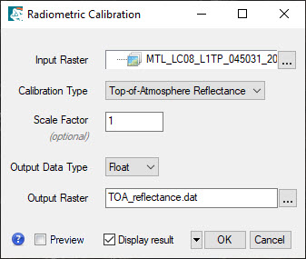
- In the Radiometric Calibration window select the data (Input Raster) for calibration, for this exercise will be using the multi spectral data "....._MTL_MultiSpectral". Set the calibration type to "Top of the Atmosphere Reflectance". Leave the default scale factor and data type (1, Float, respectively). Save the calibrated image in your Working folder as "TOA_Reflectance.dat". When the process is complete the calibrated image should automatically open.
Review: Quick Statistics
- Now we will calculate and view statistics for the image using the Quick Stats tool. Right click on the "TOA Reflectance" file in the Layer Manager and select "Quick Stats". A dialogue box will come up as ENVI calculates various statistics for the image. Once the calculations are complete the statistics view window will open.
- The basic stats include the minimum, maximum and mean pixel values for each of the bands. Scroll down to see more detailed distribution statistics for each of the bands. The values for reflectance data should range from ~0-1 (0-100%), representing 0 to 100% reflectance.
Note that there may be values outside this range that you may want to investigate. Make note if there are values greater than 1 or less than 1. Close the window when you are done.
Atmospheric Correction (Dark Subtraction)
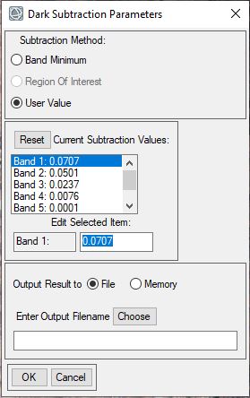
We will use the Dark Subtraction Tool to estimate and remove the effects of atmospheric scattering from the image by subtracting pixel values that represents a background scattering from each band. We will be using the band minimum
values we researched and wrote down in the previous steps.
- From the Toolbox, select Radiometric Correction → Dark Subtraction or type "Dark" in the Toolbox and open the Dark Subtraction Tool. The Dark Subtraction Correction window appears.
- In the Dark Subtraction dialog select the file "TOA Reflectance.dat" as the Input Raster and click OK.
- There are three different options for specifying the subtraction values: Band Minimum Subtraction, Region of Interest Subtraction and User Specified Values. We will use the Band Minimum method, which is the the default method. To use the Band Minimum values, don't enter or select any data in the ROI or Values options. Specify the name your output file as "Surface_Reflectance.dat" and save it in your Final Folder. Click OK to start the Dark Subtraction process, it may take a minute or two to complete the process. The image should automatically open in your viewer.
Updating Metadata and Data Ignore Values
Data ignore ( or No Data) values are pixel values that should be ignored in image processing and display. Sometimes you may need to specify the data ignore values for a raster dataset. If you have areas on your imagery that are showing up as black when they should be transparent, it means that the data ignore value is either not specified or isn’t appropriate for the data. Some processes in ENVI do not preserve the data ignore value and you may need to manually specify the value.
All of the metadata information for raster generated in ENVI is stored in an ENVI Header file (.hdr). ENVI creates a new header file whenever you save an image to ENVI raster format. The header file uses the same name as the image file, with the file extension .hdr. The data ignore value for a file is stored in the header file. You can easily edit and add metadata to these files in ENVI.
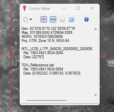
- Notice that the outside "no data' areas of the Landsat images are no longer transparent after the dark subtraction process. This is because ENVI is not properly interpreting the No Data values or the No Data value hasn't been specified. First let's check what the values of these regions are using the Cursor Value tools in ENVI. Click the Cursor Value icon on the main toolbar.

- The Cursor Value dialog contains information about the displayed data at the current cursor location, including location (coordinates) and data values for the layers turned on. Check the data values for the black, no data regions. The pixel values for these regions should be 0.
- Now let's review and update the metadata for the image (Surface Reflectance). Right click on the layer in the Layer Manager and select View Metadata. The metadata for the file will open.
- Review the metadata for the file, notice that there isn't a Data Ignore Value specified. Click the Edit Metadata button. This will allow us to edit and add metadata fields.
- The Edit ENVI Header window will open, this interface allows you to edit and add metadata fields for any file. Since there is not currently a field with the Data Ignore Value, we will need to add this to the metadata. Click the + Add button to add additional metadata fields. Select and add “Data Ignore Values”.
- At the bottom of the Main tab there will now be a field to enter in the Data Ignore Value. Enter 0 (For Landsat level-1 data the ignore values are 0, but you may need to select different values depending on the dataset). Click OK to apply.
- The image should re-load in the viewer with the data ignore values applied. The black areas should now appear transparent. We are finished processing the Level-1 Landsat imagery.
- Before moving on, let's clean-up our data to remove unnecessary files. In the main tool click the Data Manager icon. The Data Manager display all data that has been opened during the current ENVI session. Remove all of the data layers except the TOA Reflectance and final Surface Reflectance image.
- Using any program (PowerPoint, Google Slides, Canvas, Lucidchart), create a flow chart that includes the processing steps used to calibrate and correct the Level-1 data. You will include this in your lab report.Creating Flow Charts in PowerPoint. For the most effective flowchart, use different colors and symbols for
Open and Review the Level-2 Surface Reflectance Data
- Open the Landsat Level-2 data by opening up the metadata file associated with the data (LC09_L2SP_....._MTL.txt). This file is the Landsat Level-2 Surface Reflectance data that has been calibrated used the NASA/USGS algorithm (see note below). By default, ENVI will display the Level-2 Surface Reflectance Data.
Landsat 8-9 OLI Collection 2 Surface Reflectance data are generated using the Land Surface Reflectance Code (LaSRC) (version 1.5.0), which makes use of the coastal aerosol band to perform aerosol inversion tests, uses auxiliary climate data from MODIS, and a unique radiative transfer model.
- View statistics for the Level-2 image using the Quick Stats tool. Right click on the Level 2 Surface Reflectance file in the Layer Manager and select "Quick Stats". A dialogue box will come up as ENVI calculates various statistics for the image. Once the calculations are complete the statistics view window will open. Notice that there are values outside the expected range of 0-1 (0-100% reflectance), these are known computational artifacts in the Landsat surface reflectance products. For example water bodies may show negative values while bright targets such as snow and playas might display values greater than 100%. These pixel values should be masked or updated before calculating spectral indices like NDVI. Close the Quick Stats window when you are done.
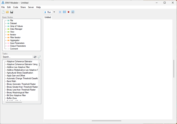
Introduction to ENVI Modeler: Automating Workflows
The ENVI Modeler is a visual programming tool that enables you to create custom task-based workflows within ENVI. The user interface is designed to help users build workflows without any knowledge of ENVI programming. You can easily create custom workflows and batch-process data with the ENVI Modeler. A model consists of two primary elements: nodes and connectors. A node is a basic building block such as an input file, task, or other operation. A connector is a grey line that connects nodes to one another via their input and output parameters. Task nodes are displayed as yellow-colored boxes, while Basic nodes are displayed as boxes of various colors (depending on your selection). If a node accepts input, it has an arrow on the left side. If it creates output, it has an arrow on the right side. A node can have arrows on both sides.
ENVI Modeler Examples from NV5 Geospatial
Examples ENVI Models from GitHub
ENVI Task List
-
We will use the ENVI Modeler to create a workflow that 'clips' pixel values outside the expected range of 0-100%. Start the ENVI Modeler using one of these options:
- Select Display > ENVI Modeler from the ENVI menu bar.
- In the ENVI Toolbox, expand the Task Processing folder and double-click ENVI Modeler. You can also drag and drop an existing .model file into the ENVI application
- The ENVI Modeler interface will open in a new window. by default, a blank model is open in the Layout Window. To begin,click the Save icon and save your model as Low High Clip in your Finals folder.
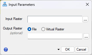
- Double-click (or drag into the model layout window) the Input Parameters under the Basic Nodes menu. The Input Parameters node creates a user interface window that opens when the model is launched, allowing the user to specify the input files and parameters to use in the model.
- Next, we will add a Task to the model. In the Tasks menu, find the Low Clip task and add it to the model window by double clicking or dragging the task into the window. To find Tasks quicker, you can type the name of task into the search bar. See the full list of Tasks available: ENVI Task List.
- Click the
 button in the Low Clip node, this will open the parameters of a node. The Low Clip task has three parameters: the Input Raster (the raster to be clipped), the Threshold (pixel values below the threshold are set to the specified threshold value), and the Output Raster (where/how the resulting raster will be saved). Close the Low Clip window for now.
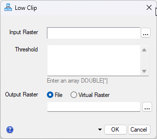
- All elements in a model need to be related with a connector. A connector is a grey line that connects nodes to one another. Connect the Low Clip node to the Input Parameters node. To connect nodes, move the cursor over an arrow in a node until a + icon appears. Click and drag to draw a line to the appropriate arrow on another node, then release the mouse button, once connected the connector becomes a solid line.
![Connect Nodes]()
- After adding this connection, the Connect Parameters window will open automatically. If more than one connection is possible between two nodes, the Connect Parameters dialog automatically appears so that you can specify the correct connection. In the window, click the Add New Inputs button under the Input Parameters and then click Input Raster. This creates an input parameter box that will allow the user to specify the raster file. Essentially, the connection feeds the user-specified raster into the Low Clip task. Click OK
![Add Inputs to Nodes]()
- Click the button in the Low Clip node to open the task parameters. The Input Raster should now be linked to the Input Parameters [input_raster], but the other parameters still need to be specified. The threshold needs to be set for each band (seven bands total for this data) as an array in the following format [0,0,0,0,0]. Set the threshold to 0 for each band (see below). This will set any pixels with negative values (less than 0) to 0. If you set parameters directly in the window, users will not be able to modify these settings.
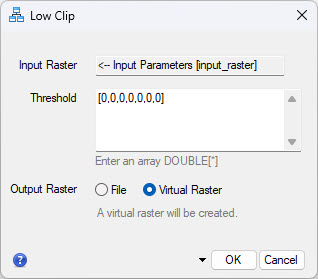
- For now, set the Output Raster to Virtual Raster. This means that the task won’t permanently save the raster. We will change this later, but to test the model, we will create virtual rasters.
What's a Virtual Raster?
Some Task nodes create virtual rasters, where no output is written to disk. Virtual rasters provide an efficient way to pass the results of one raster to the input of another task. A virtual raster is a special type of raster whose pixel values are generated on demand during data processing or visualization. Virtual rasters save time and disk space by computing only the pixels you really need instead of the entire image. They can be used as input to other operations without any intermediate steps and without having to keep track of file references.
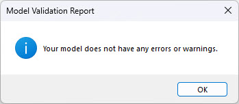
- Before moving on, we will validate the model to check for errors or missing connections. In the ENVI Modeler window select Code >Validate Model. The validation should return no errors, if not check your settings and connections and try again. Save your model.
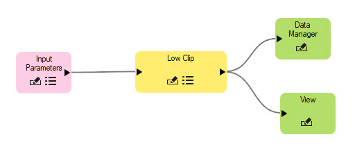
- While we could run the model now, we wouldn’t see any results because the results of the task aren't automatically added to the View or Data Manager. Use the Data Manager node whenever you create output that you want to add to the ENVI Data Manager and the View node to displays output from tasks in the current ENVI view. In the Basic Nodes menu find and add both the Data Manager and View nodes to the model.
- Connect both the Data Manager and View nodes to the output of the Low Clip node. This will send the result of the Low Clip task to the current view and add it to the Data Manager. Save your model.
- Validate your model again to make sure there are no errors or issues. Now click Run to start the model.
- An Input Parameters window will pop-up, this is where you will specify the raster to be clipped. Select the Landsat Surface Reflectance data in the Data Selection window. Then click OK to run the model.
- After the model runs you will see the newly processed image in your viewer. Use the Quick Stats tool to confirm that the Low Clip task worked. There should no longer be any negative values, the minimum bands values should be 0 for all bands.
- Now that we have confirmed that our basic models works, we will add another task and a few more parameters. Return to ENVI Modeler window (Ctrl-M is a shortcut) and add the High Clip task to the model.
- Delete the exiting connection between the Input Parameters and the Low Clip task by highlighting the connecting and clicking the Delete button or rig-clicking and select Delete.
- Connect the High Clip node to the Input Parameters node. In the Connect Parameters window, click the Add New Inputs button under the Input Parameters and then click Input Raster. Click OK to update the connection setting.
- Now connect the output of the High Clip Node to the Low Clip node. The connection window won't open this time because there is only one output from the High Clip task (the clipped raster), so the connections will automatically be set.
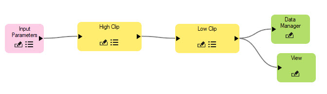
- Click the button in the High Clip node to open the task parameters. The Input Raster should now be linked to the Input Parameters [input_raster], but the upper threshold still needs to be set. Set the threshold to 1 for each band using the follow syntax, [1,1,1,1,1,1,1]. This will set any pixels with values greater than 1 to 1. Set the Output Raster to Virtual Raster and close the window.
- Validate your model to check for errors and save the model. Now the model should clip both the low (negative) and high values of the selected. Run the model and check the statistics of the resulting raster to confirm the model ran correctly.
- While to model should run correctly, it currently does not allow the user to permanently save the clipped raster or to specify the file name or location. We can add an input parameter to allow the user to specify where to save the resulting file.
- Connect the Input Parameters node to the Low Clip task node. In the Connection Parameters add a New Input that connects to the Output Raster URI button. This will create a user input field where users can specify how and where the output raster is saved. Click OK.
![Add Inputs to Nodes]()
- Now try running the model again, this time there will be an additional Input parameter . While the model works, we could improve the model by updating the labels and adding more informative help text, close the window.
- Click on the settings buttonon the Input Parameters node. In the Input Parameters window you can change the order of the inputs, alter the text and add more descriptive instructions. Update the text to make it more descriptive, e.g. Input Raster for clipping etc.
- Save your model and now run it for the final time. This time save your out put raster in your Finals folder. After running the final time, review the Quick Stats for the processed Level-2 data to ensure all values below 0 and above 1 have been adjusted.
- Use the ENVI Modeler Workflow diagram to help you create a workflow for the Level-2 data processing for your lab report. See step 20.
Comparing the Processed Level-1 Data and Level-2 Surface Reflectance Data
Now that we have finished our processing, let's compare the differences in the data products.
- In the Layer Manager select the processed Level-1 Surface Reflectance data . Click the Spectral Profile icon
 on the toolbar or select Display → Profiles → Spectral from the menu bar. This opens the Spectral Profile window. Move the cursor around to look at the spectral profiles (or reflectance curves) of different areas.
- In the Spectral Profile window click Options → Additional Profiles → Add File and select the "TOA_Reflectance.dat" and click OK. Repeat this process to added the Level-2 Surface Reflectance data (LC08 ..L2SP (Surface Reflectance)). You should now see three spectral profiles in spectral profile plot.
- In the Options menu select Legend to add a legend to the graph. Explore the spectral profile of different pixel types (i.e. Water, Vegetation, Snow, Clouds etc) by moving the cursor around the display window. Make note of any differences between the spectral profiles of the three different processed images.
- Export at least three different cover types for comparison (e.g. vegetation, water, clouds for example). Select "Export" → ASCII. This will save the data associated with the plot as a text file, the text file lists the actual pixel values (reflectance) for each of the bands, for all three images. Select "Export" → "Image" from the Spectral Profile menu bar to save a copy of the spectral profile graph. Save your spectral plot image and data in your Final folder as you will need this for your lab report, you should have three plot images and three data text files. You will need to use this data to to discuss the differences in the processing. See GSP 216 Lab 3 steps 26-34 for how to style spectral profiles and export text data into Excel.
Turn In - Summary Report
A report with:
- An overview of the data used and techniques employed.
- Two flowcharts depicting the workflow used for processing the Level-1 and Level-2 data.
- Figure showing the satellite imagery (either Level-1 or Level-2, use any color composite you wich). Include proper caption.
- Discussion: Compare the processing techniques and results for the different datasets (Level-1 and Level-2):
- Discuss the impact that the atmospheric correction (dark subtraction) had on the Level-1 data.
- How did the calibrated and corrected Level-1 data compare to the pre-processed Level-2 data? Were there differences in specific bands or certain features? Include the spectral data and graphs to back up your conclusions.
- What were the advantages/drawbacks to the different datasets?
- Completed ENVI Model file (.model)