Lab 1: ENVI and Satellite Data Review

Introduction

In this lab we will review the ENVI interface and basic data processing tasks. This lab will also review evaluating the characteristics of satellite imagery.

Learning Outcomes

• Review the ENVI user interface to open/view/export files and apply the image enhancements tools
• Establish an understanding of the data storage options, organization and file formats
• Extracting and viewing satellite images
• Exporting images from ENVI in various formats
• Review metadata, image characteristics
• Review the uses and options of the Region of Interest (ROI) tool in ENVI
• Review the use of the spectral profile tool

About the Data
The imagery in this lab exercise are two images of the Klamath River in southern Oregon and northern California. In late 2023 and early 2024, four of the six dams along the river were removed. The images from May 2023 and August 2024 show the region of the river where the Iron Gate, Copco No. 1, Copco No. 2, and J.C. Boyle dams were removed. Both images were acquired by Planet's PlanetScope Dove satellites.

ENVI 6.0
We recently upgraded to the latest version of ENVI, check out What's New in ENVI 6.0.

Accessing and Viewing PlanetScope Data in ENVI

It is important to have the files you are working with on a local drive (C: in our case). Many processes in ENVI and ArcGIS do not work well or at all when data is stored in the cloud (i.e. Google Drive G: Drive) or on portable storage devices.

1. Create a new folder on the desktop or documents folder for your lab data (recommended naming convention of the folder GSP326 Lab 1 or similar). Create two subfolders, one for the original data files and one for the final data and report.

   When you are done, you may want to back up your final work onto a USB drive, or cloud based storage like Google Drive or Dropbox or your Z: Drive ClassShare folder. The hard drives (including the desktop) on the lab computers will be deleted every 24 hours. Be sure to always save and backup your work!

2. Open a web browser, log into myHumboldt and navigate to your Humboldt Google Drive, under "Shared with Me" you should be able to see a folder for GSP 326 Intermediate Remote Sensing, there is also a link to the Google Drive folder on the Canvas home page under Resources. All of the lab data can be found in the Lab Data folder. If you are working on-campus or using vlab, the lab data can also be accessed through the ClassShare network drive (Z:) under GSP 326 > Assignments. Download/ copy the two ZIP files for this lab.
3. Extract both of the ZIP files into your original data folder, keeping the data in two separate folders. These files can now be read by ENVI.
4. Go to Start Menu and "ENVI 6.0”. This will open the ENVI 6.0 software package.
5. Once ENVI is open, go to File → Open and navigate to the original data folder. Find the folder with the 2023 data (hint - look at the file name). The PlanetScope imagery can be accessed by opening the associated metadata file. The metadata file is located in the PSScene folder. Locate and open the metadata file ending in ....3B_AnalyticMS_metadata.xml. ENVI will read the metadata file and the associated TIF file andopen the image and import the metadata. This dataset is Planet’s Surface Reflectance (SR) imagery, which is derived from the standard Planet Analytic Product (Radiance) and is processed to top-of-atmosphere reflectance and then atmospherically corrected to bottom-of-atmosphere reflectance.
6. Repeat the above process and open the 2024 PlanetScope imagery. The two image show the region of the Klamath river where the Iron Gate, Copco No. 1, Copco No. 2, and J.C. Boyle dams were located. The 2023 image was taken prior to dam removal while the 2024 image was taken recently after the last removal.
7. Use the navigation tools in the toolbar to explore the image. These tools include pan, fly, zoom. The Zoom to Full Extent Tool zooms out to show the entire extent of the image in the viewer. You can toggle the layers on and off in the layer manager to compare the two images. Spend some time exploring the images.

Visualizing Data - Compare the Images

In ENVI there are several tools that help you visualize and compare data. The Overview option shows a thumbnail of the raster and defines the extent currently shown in the view. Another useful tool is the Reference Map Link that opens up a new window with a variety of base maps that correspond to the raster in the viewer.

8. Click the Overview check box for the desired View in the Layer Manager window. The Overview appears in the top-left corner of each Image window view. The Overview Locater, a rectangle within the Overview, defines the extent to show in the view. As you move around the image the locator rectangle moves accordingly. Turn off the Overview by clicking the disable the check box.
9. Now let’s get an idea of the geographic area the images cover. From the menu bar select View → Reference Map Link. This opens up a new window with a variety of base map options that shows the geographic extent of the raster in the viewer.
10. The Blend, Flicker and Swipe tools that can be used to compare layers. These are found in the main toolbar . First click on the "Blend" icon in the toolbar . This creates an animation that blends or fades between the two selected layers. Click on the "Flicker" icon in the toolbar. This creates an animation that switches between the two layer. Finally click on the "Swipe" icon in the toolbar. This creates an animation that swipes between the two layer. Use these tools to compare the two images.



In ENVI by default the image window displays data layers in a single view. You can add up to 16 views containing different files. You can also link multiple image window views by geography so when you zoom or pan in one view the other views automatically follow.

11. From the main toolbar, select Views → Create New View to open a new view in the image window. Drag and drop one of the images from the Layer Manager into the new view. By default the views are not linked and can be moved independently
12. Using the Link View tool, you can link up to 16 views (or windows) by geographic location so that all linked views will go to the same location at the same time when you pan/zoom around the image. From the main menu, select Views → Link Views. Select “Geo Link” and then click the “Link All” button. This links all open views. Click “OK”. Now when you zoom or pan in one view the other views automatically follow. Now you can compare the images side-by-side. when you are done comparing the images side-by-side you may close the second view if you like or keep it open (your choice).

Review Metadata

Metadata provide details about a dataset in general such as its source, data type, and projection. In ENVI the metadata is stored in the header file (.hdr). The metadata can be edited in the program or the header file can be edited using a text editing program like notepad.

13. Open the Metadata Viewer by right clicking on the file name in the Layer Manager and selecting "View Metadata". Click through the various tabs and explore the metadata. Use the metadata viewer to determine the spatial and spectral resolution of both of the image as well as the projection/coordinate system. Record this information as you will need to include in your lab submission.

Image Display Options

Changing Band Combinations

ENVI 6.0 includes the new Dynamic Band Selection tool, which allows you easily change the RGB band combination for the selected raster in the view. The Dynamic Band Selection controls appear at the bottom of the Layer tab when a raster file is open. This tool replaces the Change RGB Bands option that was previously available in the right-click menu of the Layer Manager.



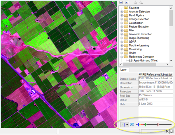
14. Select one of files in the Layer Manager and navigate to the Layer tab in the lower right hand corner. This is where the band selection tool is now located. Start by selecting different preset band combinations from the list, to do this, click the drop-down arrow next to the sliders . Try a few different preset composites.
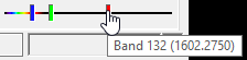
15. Now try selecting your own band combinations. To make your own band combinations, click and drag the slider bars for red, blue, and green to select the bands to use for each display color.
16. Select what ever composite you would like to move forward with or stick with a true color composite. You can always change this at any time.

Image Enhancement Controls

Enhancement tools interactively control the amount of brightness, contrast, stretch, and transparency for the selected image layer. For each tool you can click and drag the slider, or enter a value in the adjacent field. You can control the Brightness, Contrast, Sharpness and Transparency. You can also apply different stretch types to enhance the appearance of an image.

17. Explore the Brightness, Contrast, Sharpness and Transparency image enhancements controls for the images. Setting can be reset to the defaults by clicking the reset icon. Use these tools to visualize and compare the images.
18. Locate the Contrast Stretch drop-down in the main toolbar and try all of the different contrast stretches. If you are unhappy with the contrast stretch you can always click the "Reset Stretch Type" icon to restore the contrast to the default setting. The Custom Contrast Stretch also allows you to apply custom contrast stretches using the histograms as a guide. This tool allows the user to set the minimum and maximum value for each color channel (Red, Green, Blue) that the contrast stretch is applied. Experiment with the different contrast stretch types and select one (either custom or pre-set). Do this for both of the images.

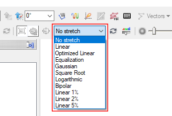
Spectral Profiles

Now we will use the spectral profile tool to compare the spectral profile of a pixel before and after the dam removal.

19. Click the Spectral Profile icon on the toolbar or select Display → Profiles → Spectral from the menu bar. This opens the Spectral Profile window and by default it plots the spectral profile of the pixel in the center of the screen of the selected data file.
20. Now we will add a profile for the other dataset (whichever isn't currently shown). In the Spectral Profile window click Options → Additional Profiles → Add File and select the other image file and click OK. You should now see two spectral profiles, one for the 2023 image and one for the 2024 image.
21. Compare the spectral profiles for avarious locations near the dam removals sites. Select one location to create and export a spectral profile chart. Your spectral profile chart should show the two profiles, one for 2023 and the other for 2024. Add a legend and update the names and axis as appropriate and export your spectral profile chart as a JPG. See GSP 216 Lab 3 and Lab 8 for reference.

Measuring Features

If an image is georeferenced to a standard map projection, you can measure the distance between objects using the Mensuration tool in ENVI. This is an easy way to quickly track and measures changes in the landscape. The Region of Interest Tool (ROI) is an excellent tool to map and measure area.

Measure Linear Distances

22. Use the "Go To" tool in the main toolbar to jump to a specific location in an image and to center the current image window view over that location. Enter the following coordinates in the Go To field: 41.934364, -122.436145 and press enter. These coordinates are the rough location of the Iron Gate dam.
23. Use the Mensuration tool to measure the distance across Iron Gate dam using the 2023 image. Click the Mensuration button in the toolbar. Red cross-hairs appear in the display, and the Cursor Value dialog appears. Click on the first point to start the measurement and drop a subsequent points to measure a distance. Right click and select accept.
24. The measurement will show up as an Annotation. You can see the measurement value in the Cursor Value menu and you can change the measurement units as you see fit. Write down or copy the measured valued. Close the cursor value window when you are done. You can uncheck the annotation or remove it in the Layer Manager if you would like.

Create ROIs and Calculate Area

Regions of Interest (ROIs) allow you to select specific areas of rasters. The ROIs can be saved and used for a variety of purposes, including calculating statistics, area and subsetting images. ROIs can be created from geometry or by pixels. ROIs are vector files, which are coordinate-based data models that represent geographic features as points, lines, and polygons. While ROIs are an ENVI data type, they can also be exported as Shapefiles.

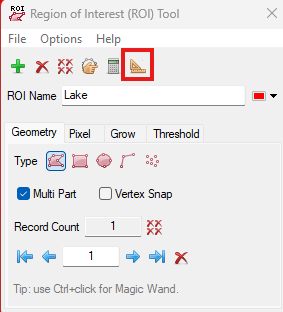
25. Now we will map and measure the area of the two reservoirs (Iron Gate and Copco). If necessary change the band combinations to a false color composite that makes water stand out. Right-click on the 2023 file in the Layer Manager, and select New Region of Interest. Create a Multi Part Polygon ROI and name the ROI appropriately.
26. We will use the Magic Wand tool to grow ROI polygons from one or more "seed" pixels. This tool facilitates drawing ROI polygons around complex objects such as clouds, tree crowns, and lakes. With the Region of Interest (ROI) Tool displayed, hold down the Ctrl key and click on a pixel inside of water. An initial polygon is drawn, and the Magic Wand Parameters dialog appears. You can adjust the threshold and experiment with other parameters to better refine the shape of the object. Try checking and unchecking the Use Pyramids option and see how the area changes.
27. Add additional areas to the ROI by holding down Ctrl key and clicking a the new region. Once you are happy with your ROI selection (aim to select the entire lake area but no other features), right click and select "Accept Multipart". Click the area icon in the lower half of the ROI window and record the area in either acres or hectares. See GSP 216 Lab 5 for review.
28. Now create new ROI and repeat the process for the other reservoir, be sure to record the area. You should now have two ROIS, one covering each of the reservoir. You may export the ROIs as shapefiles if you want to create maps of figures in ArcGIS or save in the ENVI ROI format for future use.

Export Images

29. Using the display options, adjust your images and layers to create three figures. Your figures should show the 1) 2023 image, 2) 2024 image and the 3) 2024 image with the two ROIs overlayed on the layer. You may use any color composite that you like. When including the ROIs, I recommend adjusting the transparency of the ROIs for visual effect. Use the "Chip to View" option in ENVI to save the current view as an images that can shared or placed in a report. This option is very similar to taking a screenshot. To Chip a View Go to File > Chip View To >File in ENVI. Select "JPEG" as the output file type and uncheck "Display Results."
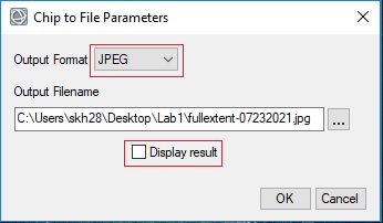
30. Repeat the process for the other images. The views will export exactly how they look on the screen in terms of zoom and size. For other export options see Saving and Export in Files in ENVI. Close ENVI when you are happy with your exported images.
31. Back up your Finals folder. I recommend zipping the folder and then transferring to Google Drive or a USB storage device.

Turn In

(1) A Word document with:

• Table showing the spectral/spatial resolution, date, sensor and projection/coordinate system of each of the images.
• Spectral Profile graph comparing the 2023 and 2024 reflectance profiles for a location
• Figure (3) showing the 2023 image, 2024 image and the 2024 image with the ROIs
• The approximate linear distance across the Iron Gate Dam
• The area in acres or hectares of Iron Gate and Copco Reservoir.