Lab 7 - Part 2: More Lidar in ArcGIS Pro
Introduction
This exercise is a continuation of Lab 7 Part 1 - Working with Publicly Available Lidar in ArcGIS Pro. The same lidar dataset of Montgomery Woods will be used and the raster products created in the previous exercise will also be used. This lab exercise will focus on visualizing the lidar derived data products and extracting further information from the lidar data.
About the Data
This data is lidar points clouds data available through the USGS 3D Elevation Program through the National Map. The area of interest is Montgomery Woods State Natural Reserve in Mendocino County. The reserve originated with a nine-acre donation by Robert Orr in 1945 and has since been enlarged to 2,743 acres by purchases and donations from Save the Redwoods League. A 367.5-foot redwood at Montgomery Woods was once thought to be the tallest tree in the world. Taller trees have since been found in Humboldt Redwoods State Park and Redwoods National Park, but Montgomery Woods is still noted for its lofty giants. The lidar data was collected in 2016.
View Data in 3D
- Copy your data from the previous Lab from Z: or Google Drive to your local workstation. Open ArcGIS Pro and open up the previous map projecty with the Montgomery Woods lidar.
- Let's spend some time exploring the 3D viewing options. Click on the existing 3D scene you created in the previous lab exercise or convert an existing 2D scene into a 3D (Local Scene)
- Check out the LASD layer first. In the 3D view you can see all points and pan/move the area around. You can control the display of the LAS points in the 3D map the same as you can in 2D. Play around with the data and navigation. Turn off the LASD layer when you are done looking at it. This will speed up the rendering times.
- Right-click on the Ground element under the Elevation Surfaces group at the bottom of the Content Pane and select Add Elevation Source. Select the DEM.tif and DSM.tif rasters from the project folder then click OK. Remove the default "WorldElevation3D/Terrain3D" layer.
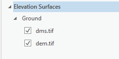
- Any layer added to the 2D layers group will be draped over the elevation surface. Note that the DEM is the bare ground elevation and terrain, while the DSM includes the elevation of the above ground vegetation in addition to the ground. Turn the two elevation surface layers on and off to see the differences between the two.
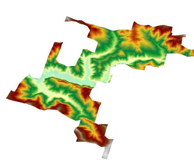
- Now add the Imagery Basemap to your 3D map. This will display a recent satellite or aerial image or the area. Try turning on and off the different layers and experimenting with the display options. Turn on the various height model rasters and see how they look in the 3D scene. For more information on navigating in scenes and linking scenes check out the Navigate maps and scenes in ArcGIS Pro video. Either stay in the 3D scene or return to the 2D scene for the next steps.
Locate the Trees Greater than 350ft Tall
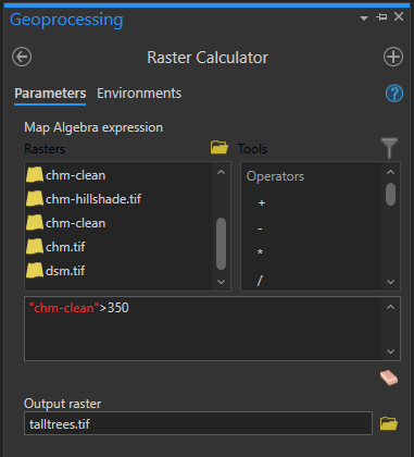
- Use the Raster Calculator to locate the trees with canopies greater than 350 feet tall. Use your final cleaned up CHM layer in the raster calculator expression. The result should be a binary raster, with ‘1‘ values indicating canopy greater than 350 ft.
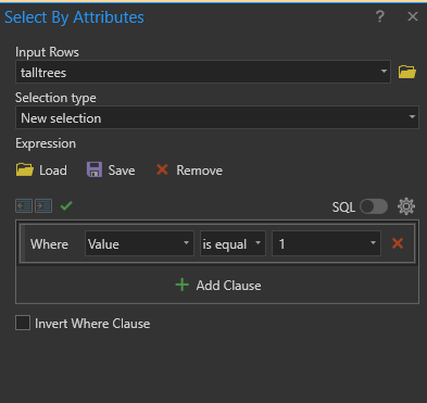
- Open the Attribute Table for the “talltrees” layer you just created and select the row containing the “1” values. The pixels with 1 values should now be highlighted light blue on the map. You could also use the Select by Attribute function to select the pixels where the value field is equal to 1.
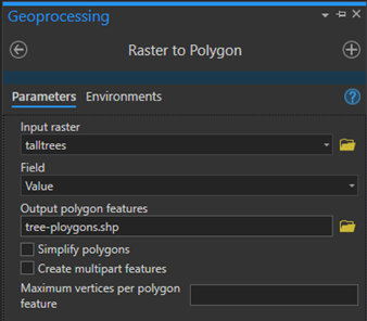
- Take a look at the results and compare the pixels to the canopy height model. Notice that the pixels are grouped together and several pixels represent an individual tree. Now we will create polygons from these selected pixels so each group of pixels is grouped together into a single polygon. Run the Raster to Polygon tool to accomplish this. Select the “talltrees” as the input file from the drop down. Field should be set to Value and save the polygon as tree-polygon.shp and run the tool.
- Now we have a shapefile with polygons showing the locations of the tallest tree canopies. For visualization and mapping purposes we will also create a point shapefile showing the locations of the tallest trees. To do this run the Feature To Point tool. Select the tree polygons as the input feature and name the outpost feature class as tree-points.shp and run the tool.
- We now have the locations of the tallest trees. Review your final locations and cleaned-up tree-points layer removing any erroneous or duplicate points. If you make any edits you will need to save your edits (under the Edit tab in the main toolbar) before completing the last steps.
- Create a slope layer from the DEM file using the Slope geoprocessing tool or using the Raster Function
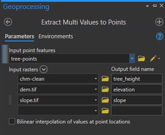
- The Extract Multi Values to Points tool extracts pixel values at point feature location from one or more rasters and records the values to the attribute table of the point feature class. Under input rasters add the canopy height, elevation (dem) and slope value. Then run the tool.
- You should now have a point feature layer that includes the elevation, height and slope attributes of the locations of the tallest trees. Open the attribute table for the point layer.
- The last thing we will do is to add the XY coordinates of the points to the attribute table. Run the Calculate Geometry Attributes geoprocessing tool. Select the tree-points layer as the input feature. We will add two new fields for the latitude and longitude (see below). The latitude is the y coordinate and longitude the x-coordinate. Select Decimal Degrees as the coordinate format and Current Map for the coordinate system and run the tool. Now the coordinates have been added to the attribute table. Copy the information from the attribution into a spreadsheet.
Find the Highest and Lowest Elevation
- Using some of the same above methodology (steps 2-4) find the lowest and highest elevation areas in the reserve and create a point feature that shows the locations. Consider using the Raster to Point Coversion tool rather than the Raster to Polygon to simplify the process.
Create Hillshades and Maps
-
Create hillshades for the CHM, DEM and DSM. You can either use the Raster Functions tool to generate a hillshade on the fly (no file is saved) or use the Hillshade geoprocessing tool to save a hillshade for each layer. These will be used to create the final maps.
- Create two maps, one showing the canopy height model and one showing the elevation. Both maps should use the approriate hillshades to provide relief shading. The elevation map should display the bare earth terrain, elevation color ramp and the low and high elevation location. For the canopy height map use either the DMS or CHM hillshade, the canopy height in color and optionally the locations of the tallest trees.
Turn In