Lab 3: Image Statistics and Data Processing

Introduction

In this lab we will cover the ENVI processing techniques for layer stacking and masking. This lab will also cover reviewing image statistics and histograms.

Learning Outcomes

• Open and evaluate Sentinel-2 data
• Perform Layer Stacking operations
• Evaluating Image Statistics
• Creating and Applying Masks
• Comparing and extracting data

About the Data
The primary data in this lab is Sentinel-2 Level2A data. This is data has been processed to bottom of the atmosphere (BOA) reflectance, (or surface reflectance). The specific image used in this lab was acquired August 2023 over western British Columbia, Canada.

Accessing Sentinel-2 Data in ENVI

1. Create a new folder on the desktop or documents for your lab data (recommend naming convention of the folder “GSP326_Lab_#”). Create two subfolders, for original files, and final processed files.
2. Open up your favorite web browser, log into myHumboldt and navigate to your Humboldt Google Drive, navigate to the Lab 3 Data folder and download the Sentinel-2 ZIP file.
3. Extract the files into your original data folder. Note that you may need to rename the Sentinel-2 ZIP file to a shorter name, as the file names can be too long. When the extracting process is finished you should have a series of folders that contain various data files. Open ENVI.
4. In ENVI, select File → Open and navigate to your Originals folder where you extracted your data and find the folder that contains the Sentinel-2 data. Open the metadata XML file that begins with "MTD_MSI...".
5. You should now see the true color Sentinel-2 image. ENVI will automatically display the 10m resolution true color view of the scene and the other bands (20m and 60m) files will be available in the Data Manager.

   Band Number	Central Wavelength (nm)	Bandwidth (nm)	Spatial Resolution (m)
   B1	443	20	60
   B2	490	65	10
   B3	560	35	10
   B4	665	30	10
   B5	705	15	20
   B6	740	15	20
   B7	783	20	20
   B8	842	115	10
   B8a	865	20	20
   B9	945	20	60
   B10	1375	30	60
   B11	1610	90	20
   B12	2190	180	20

6. Spend some time looking at the different bands available in the data manager. The bands are packaged in "bundles" based on resolution and data type. See the below table for reference. You can select different band combinations and add them to your viewer.

Bands	Description
10m-S2MSI	Surface reflectance for 10m bands (RGB, NIR)
10m-AOT	Aerosol optical thickness (unitless)
10m-WVP	Water vapor
10m-TCI	True color image - an RGB image built from the B02 (Blue), B03 (Green), and B04 (Red) Bands. The reflectance are coded between 1 and 255
20-SCL	Scene classification data at 20m resolution

7. Now we will create a Layer Stack to create one raster that includes the first 10 bands of the data in one file (the 10m and 20m resolution data). In the Toolbox select Raster Management → Build Layer Stack.
8. In the Layer Stack window click to add the layer beside Input Rasters. In the Data Selection Window select the 10 and 20m data (hold Ctrl key to select multiple items). Click OK.
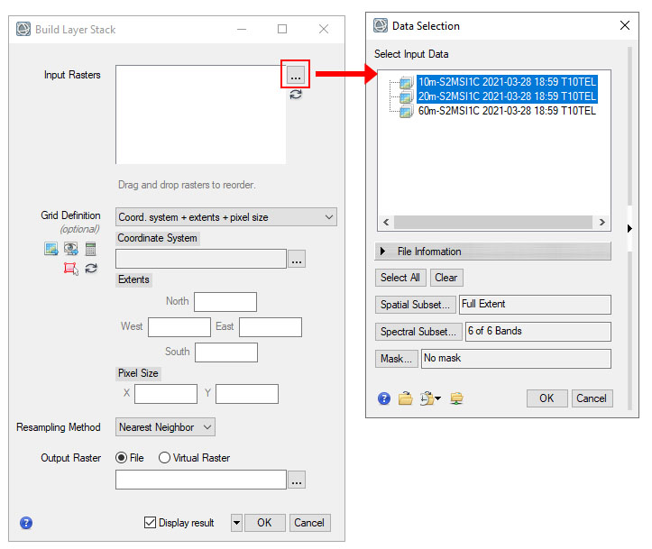
9. In the main Layer Stack dialog, under Grid Definition select From Dataset. Select the 20m Sentinel data file as the reference dataset. This will set the coordinate system and cell size based on this dataset. Click OK.
10. In the main Layer Stack dialog save your output Layer Stack file as Sentinel_stack.dat in your finals folder. This file will contain the first 10 bands of the Sentinel-2 data. Click OK to create and save the layer stack. Wait to the image to load and for the pyramid layers to fully load. The stacked image should appear in your viewer when the process is complete.

View Image Statistics and Histograms

11. Now that we have a layer stack with all of the desired bands, we will calculate and view statistics for the image. In the tool box select Statistics → Computer Band Statistics.
12. In the Compute Statistics input file select the Sentinel-2 stack you just created and click OK.
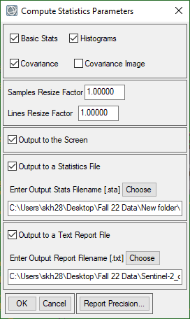
13. In the parameters windows select Basic Stats, Histograms, Covariance. Check the boxes to Output the data to the screen as well as a Statistics File and Text File. Save the Statistics (.sta) and text file (.txt) in your finals folder. Click OK to run the statistics.
14. Check out the statistics on the screen. The basic stats include the minimum, maximum, mean and standard deviation for each of the bands. Scroll down to see more statistics and detailed distribution statistics for each of the bands. The values for reflectance data should range from ~0-10000, representing 0 to 100% reflectance. Note that there may be values outside this range that you may want to investigate.
15. Below the basic stats are the correlation and covariance tables showing the relationship between bands. All of this same data is also included in the statistics text file (.txt) you save in the previous steps. In windows explorer, find the text file that you save and open in notepad or similar text reader. Review the stats in the text file.
16. Now we will view the histograms for all of the bands. In the upper left hand corner click "Select Plot" and select "All Histograms". Look at the distribution and shape of the histograms. You can save the histogram by selecting Export → Image. Also check out some of the other plots available. Close the Statistics Windows when you are done. You may need to revisit some of this information to complete the worksheet.

Investigate Low and High Pixel Values

Use the ROI threshold tool or the Raster Color slice tool to investigate various pixel values in the image.

18. Create a new ROI on the Sentinel-2 stack. Use the ROI threshold tool to find the features in the image with the lowest overall reflectance (across all of the bands) and the highest overall reflectance. Make note of what and where these features are in the image.
19. Now try using the raster color slice tool to investigate specific values in the images. Right click on the Sentinel stack layer and select New Raster Color Slice. Select the band you want to use to create a color slice. Specifically locate features that have greater than 100% reflectance in a band.
20. Review the worksheet questions. Answer the questions based on the statistics files and the above investigations.

Create ROI and Raster Mask for Specific Features

Now we will create a few masks for our image in preparation of image classification (next week).

21. Create a ROI to use as a mask for the no-data areas of the image. See Lab 2 steps 15-17 for a refresher on how to create a ROI that includes only the no data areas of an image.
22. Similar to the Landsat QA bands, the Sentintel-2 Level-2 data includes a scene classification layer. This is the automatically generated scene classification data, based on ESA Sen2Cor processor (the algorithm that performs atmospheric and terrain correction on the data). Open the Data Manager and load the data labeled 20m-SCL....
23. Check out the layer and associated classes. This layer can be used similarly to the Landsat QA band. We will use it to create a few masks for the dataset.
24. Create a new ROI and in the ROI Tool, click the Threshold tab. Click the Add New Threshold Rule button . In the File Selection dialog, select the SCL classification band and click OK.
25. Try creating two different masks, one that only includes vegetation (no clouds/snow/water etc) and one that only includes water and snow (no clouds, vegetation etc). For these mask you will want to have the ROI cover the areas that you want masked.
26. Use the Min and Max values or the histogram to select all of the appropriate features. You may need to add more than one threshold rule depending on the values you need to select. Check the preview box to see the areas selected by the range of values. Click OK when the appropriate areas are selected. Use the preview option on the screen to make sure that your
27. Save the ROIs for futures use (in another work session), by selecting File > Save As and save the selected ROI as an XML file.
28. Now we will also create a binary raster mask from the ROI. From the Toolbox, select Raster Management > Build Raster Mask. The Build Mask Input File dialog appears.
29. Select the input file of Sentinel stack and click OK. The Mask Definition dialog appears. More information about creating masks in ENVI and how they can be applied »
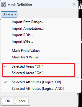
30. From the Mask Definition dialog menu bar, select Options and select the ROIs you made in the previous steps to include in the mask. Make sure the selected areas are "OFF" under the options. This means areas highlighted by the ROI will be masked.
31. After adding the ROI, name the file as type of mask.dat (update the file name depending on the type of mask you are creating) in the final folder and click OK. Repeat this process so you now have two saved mask rasters (.dat files).
32. Now that we have our masks we can easily apply them. We will calculate and view statistics for the image again but this time we will apply a mask in the Calculate Statistics tool. In the tool box select Statistics → Computer Band Statistics.
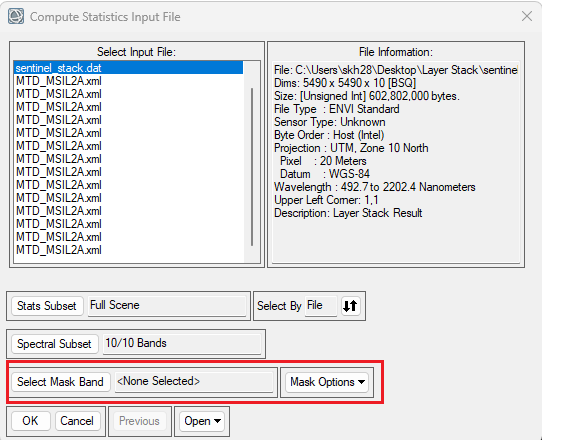
33. In the Compute Statistics input file select the Sentinel-2 stack you just created but be sure to select a Mask Band before moving to the next steps. Select one of the mask you just created and then click OK. Compute the same statistics as you did in previous steps (12-13) and save the statistics files. Make sure to give the statistic file a unique file name indicating that the stats are for masked areas.
34. Back up your folder. We will need this data for next week's lab.

Turn In - Worksheet and Text file

Upload to Canvas

• Completed Lab 3 Statistics Worksheet
• ENVI generated statistics text file for the Sentinel-2 data stack (.txt).
• ENVI generated statistics text file for the masked Sentinel-2 data stack (.txt). Indicate what mask was applied (snow/vegetation).