Lab 2: Image Processing Techniques in ENVI
Introduction
In this lab we will cover the ENVI processing techniques for radiometric calibration, atmospheric correction and masking. This lab will also cover applying masks and calculating spectral indices.
Learning Outcomes
- Perform Radiometric Calibration in ENVI
- Conducting atmospheric correction (dark object subtraction)
- Evaluating Image Statistics
- Creating and Applying Masks
- Comparing and extracting data
- Calculating Spectral Indices
- Visualizing Data
About the Data
The primary data is this lab is Landsat Collection 2 Level-1, Landsat Collection 2 Level-2 Surface Reflectance data will be viewed for comparison.
The specific data used in the lab is a Landsat 8 image of northern California and souther Oregon acquired July 8th 2023.
Accessing and Calibrating Landsat Data in ENVI
You will begin by creating a folder structure or "workspace" that will keep your files organized and prevent any confusion as you work with multiple datasets in the future. It is important to have the files you are working with on a local drive (C: in our case). Many processes in ENVI and ArcGIS do not work well or at all when data is stored in the cloud (i.e. Google Drive G: Drive) or on portable storage devices. Back up your data when you are done!
- Create a new folder on the desktop or documents folder for your lab data (recommended naming convention of the folder “GSP326_Lab_#”). Create three subfolders: original files, working and final.
When you are done, you will want to back up your final work onto a USB drive, or cloud based storage like Google Drive or the Course Share Z: Drive. The hard drives (including the desktop) on the lab computers will be deleted every 24 hours. Be sure to always save and backup your work!
- Download the Lab 2 data files from the shared Google Drive folder or the class share network drive (Z:). The data consists of two Landsat "tarball" files (.tar).
- Use 7-Zip to extract the two files into your original data folder, note that each of the files should be extracted into separate folders. When the process is finished you should have two folders that each contain Landsat data files, one is Level-1 data while the other is Level-2 data.. Open ENVI (ENVI 5.6.X). This will open the ENVI software package.
- In ENVI go to File → Open and navigate to the location of the Lab 2 original data folder. Find the folder with the Level-1 Landsat 8 data (hint: look at the file name, level-1 data os desognated with L1TP) and select the metadata text file (it will end in "_mtl.txt") and click open.
- First we will calibrate the Level-1 data so the pixel values represent real-world units, in this case percent reflectance. From the Toolbox, select Radiometric Correction → Radiometric Calibration or type “radiometric” in the toolbox and open the Radiometric Calibration tool.
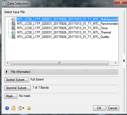
- In the Radiometric Calibration window we need to select the data for calibration, select the Landsat 8 multispectral image, it will end in "....._MTL_MultiSpectral" and click OK. This will radiometrically calibrate the seven reflective, multispectral bands of the Landsat 8 data.
- In the next window select "Reflectance" as the calibration type and keep the other default settings. Save the calibrated image in your Working folder as "TOA_Reflectance.dat". TOA stands for Top of the Atmosphere, as this is the reflectance measured at the top of the atmosphere at the sensor (which includes the effects of atmospheric scattering). When the process is complete the calibrated image should automatically open.
View Image Statistics
- Now we will calculate and view statistics for the image. Right click on the "TOA Reflectance" file in the Layer Manager and select "Quick Stats". A dialogue box will come up as ENVI calculates various statistics for the image. Once the calculations are complete the statistics view window will open.
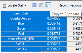
- The basic stats include the minimum, maximum and mean pixel values for each of the bands. Scroll down to see more detailed distribution statistics for each of the bands. The values for reflectance data should range from ~0-1, representing 0 to 100% reflectance.
Note that there may be values outside this range that you may want to investigate.
- For each band (seven in total) write down or copy/paste the minimum value, this is the lowest (non-zero) pixel value for that band. You can highlight the Band and associated Min value columns and copy them by selecting the Copy to Clipboard icon, then paste this information into a spreadsheet. We will use this information for our atmospheric correction process (note that values will differ from image below).
Atmospheric Correction (Dark Subtraction)
We will use the Dark Subtraction Tool to estimate and remove the effects of atmospheric scattering from the image by subtracting pixel values that represents a background scattering from each band. We will be using the band minimum
values we researched and wrote down in the previous steps.
- From the Toolbox, select Radiometric Correction → Dark Subtraction or type "Dark" in the Toolbox and open the Dark Subtraction Tool. The Dark Subtraction Input File window appears.
- In the Dark Subtraction Input File dialog select the file "TOA Reflectance" and click OK.
- The Dark Subtraction Values dialog appears, under Subtraction Method select "User Value". Click on each band (Bands 1-7) and enter in the minimum value you wrote down in the previous steps. Once you have entered in a value for Band 1, click on Band 2 and enter in the appropriate value. Do this for all seven bands. Note the image below is an example and that values will differ.
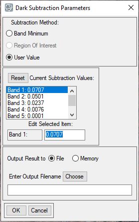
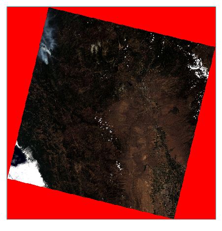
- Once you have entered in the values for all seven bands name your output file "surface_reflectance.dat" and save it in your Final Folder. Click OK to start the Dark Subtraction process, it may take a minute or two to complete the process. The image should automatically open in your viewer.
Masking with ROIs - Create a No Data Mask
Masks are used to exclude certain pixels from image processing or when computing image statistics. Masked pixels appear as transparent in the display. Masks can be created several different ways, using the FMask tool, ROIs or the Build Raster Mask Tool. The next steps will go over several methods.
- Notice that the outside "no data' areas of the Landsat images are no longer transparent after the dark subtraction process. We can apply a mask to properly exclude these values from display and analysis. Right-click on the Surface Reflectance file in the Layer Manager, and select New Region of Interest. Name the ROI no-data in the ROI tool window.
- In the ROI Tool, click the Threshold tab. Click the Add New Threshold Rule button
 . In the File Selection dialog, select the first band associated with the Surface Reflectance file and click OK. A histogram of the band is displayed in the Choose Threshold Parameters dialog.
- Use the Min and Max values or the histogram to select all of the 'no data' areas outside the image. These values should be negative. Check the preview box to see the areas selected by the range of values. Click OK when the appropriate areas are selected. If you want to save the ROI for futures use (in another work session), select File > Save As and save the selected ROIs as an XML file that can be read by ENVI.
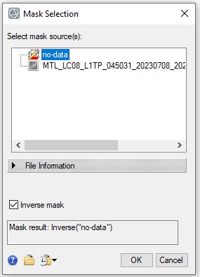
- We will now use the ROI to mask the image. To apply the mask we will use the Save As operation to create a new files with the no-data areas masked. In the Main toolbar, select File → Save As → Save As.. (ENVI). In the Data Selection Window select the "surface_reflectance" as the Input File. Click the Mask button below. In the Mask Selection Window select the "no-data" ROI and check the inverse mask button, then click OK. Click OK in the Data Selection window to save the file. Note that the default is to mask the areas outside of the ROI, if you would like to mask the area selected by the ROI the inverse mask button should be checked.
- Set the data ignore value to 0 and save the file as SR_masked.dat in your final folder. When the new image appears the "no data" areas should be hidden.
Compare the Data Processed Level-1 Data to the Level-2 Surface Reflectance Data
- For comparison open the Landsat Level-2 data by opening up the metadata file associated with the data (LC08_L2SP_....._MTL.txt). This file is the Landsat Level-2 Surface Reflectance data that has been calibrated used the NASA/USGS algorithm (see note below). We will use this data to compare it to our processed data.
Landsat 8-9 OLI Collection 2 Surface Reflectance data are generated using the Land Surface Reflectance Code (LaSRC) (version 1.5.0), which makes use of the coastal aerosol band to perform aerosol inversion tests, uses auxiliary climate data from MODIS, and a unique radiative transfer model.
- In the Layer Manager make sure your have the masked Surface Reflectance data selected. Click the Spectral Profile icon
 on the toolbar or select Display → Profiles → Spectral from the menu bar. This opens the Spectral Profile window. Move the cursor around to look at the spectral profiles (or reflectance curves) of different areas. The x-axis is the the wavelength and the y-axis displays the percent of light reflected (
- In the Spectral Profile window click Options → Additional Profiles → Add File and select the "TOA_Reflectance.dat" and click OK. Repeat this process to added the Level-2 Surface Reflectance data (LC08 ..L2SP (Surface Reflectance)). You should now see three spectral profiles in spectral profile plot.
- In the Options menu select Legend to add a legend to the graph. Explore the spectral profile of different pixel types (i.e. Water, Vegetation, Snow, Clouds etc) by moving the cursor around the display window. Make note of any differences between the spectral profiles of the three different processed images.
- Export at least three different data points for comparison (e.g. vegetation, water clouds for example). Select "Export" → ASCII. This will save the data associated with the plot as a text file, the text file lists the actual pixel values (reflectance) for each of the bands, for all three images. Select "Export" → "Image" from the Spectral Profile menu bar to save a copy of the spectral profile graph. Save your spectral plot image and data in your Final folder as you will need this for your lab report, you should have three plot images and three data text files. You will need to use this data to to discuss the differences in the processing. See GSP 216 Lab 3 steps 26-34 for how to style spectral profiles and export text data into Excel.
Masking Specific Features
You can create a mask from a region of interest (ROI), from a shapefile, by creating binary rasters, or by using options available in the Build Raster Mask tool. In addition to excluding the no data areas, we also want to exclude water and cloud pixels from a vegetation analysis. There are many different ways to create clouds (and other feature) masks and the next section will cover a few techniques.
Fmask Algorithm Cloud Mask
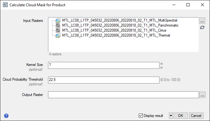
- The Calculate Cloud Mask Using Fmask tool can be used to create a cloud mask for Landsat and Sentinel-2 data. We will test out the tool on out dataset. From the Toolbox, select Feature Extraction > Calculate Cloud Mask Using Fmask Algorithm.
- Click the Browse button next to the Input Rasters field. In the File Selection dialog, select all datasets that correspond to the Landsat Level-1 files and click OK in the File Selection dialog.
- Keep all of the default parameters. Select the working folder as the output file location and name your file Fmask.dat. Check the Display result option and click OK to run the process.
- When processing is complete, the cloud mask is displayed and added to the Layer Manager. The cloud mask is a binary image where cloud (masked) pixels have values of 0 and non-cloud (non-masked) pixels have values of 1. Visually evaluate the effectiveness of the Fmask process by toggling the layers. Note what features are included in the mask and which are not.
View the Landsat QA Band
Landsat data products also include Quality Assessment (QA) bands to identify the pixels that exhibit adverse instrument, atmospheric, or surface conditions. This can include clouds, cloud shadows. This information can also be used to generate masks to exclude or isolate certain pixel types from analysis. There are several external tools available to extract information from the QA bands : https://www.usgs.gov/landsat-missions/landsat-level-1-quality-assessment-tools
- Now we will open the Landsat QA band, select file open and in your Originals folder and select the file "LC08_L1TP_.....QA_PIXEL.tif" and click OK. This is the Landsat Quality Assessment band.
- Use the cursor value tool
 to investigate what some of the pixel values are for various features (clouds water etc). You may want to open a new view or toggle between the Landsat surface reflectance layer and the QA band layer for comparison. Make note of some of the QA pixel values associate with clouds, shadows and other features that you might want to mask.
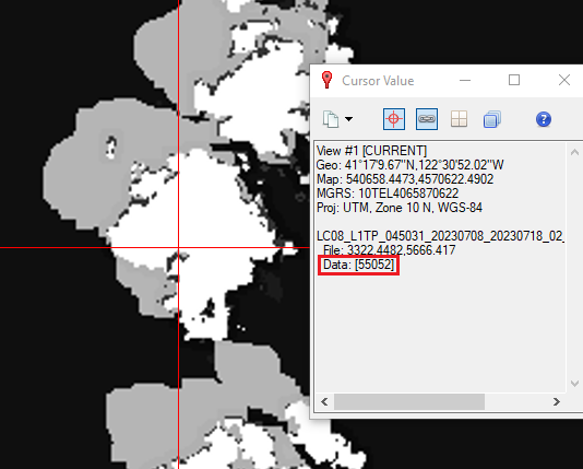
- Now we will create a ROI (Region of Interest) to use as out mask. Multiple ROIs can be employed to create a mask. Right click on the SR_Masked.dat file and select New Region of Interest. Use the threshold option to select certain pixel values in the ROI. Experiment using different bands and the QA bands to try and isolate certain features in the image. For example clouds tend to have relatively high reflectance across the spectrum while water and cloud shadows have low reflectance. Depending on the scene and masking requirements you may want to create multiple separate ROIs for different features. You can also create multiple threshold rules for an ROI.
-
You can also use the following steps for the Build Raster Mask tool to create a binary raster from specific pixel values or ranges of pixel values or by selecting ROIs to create the mask. From the Toolbox, select Raster Management > Build Raster Mask. The Build Mask Input File dialog appears.
- Select the input file of SR_masked.dat and click OK. The Mask Definition dialog appears. From the Mask Definition dialog menu bar, select Options, here you can choose to add specific values to mask or ROIs to include in the mask. Under options select the import ROIs option and add the ROI(s) you created in the previous setp. If the input file has a data ignore values (no data values), then the dialog opens with these values automatically entered in these fields.
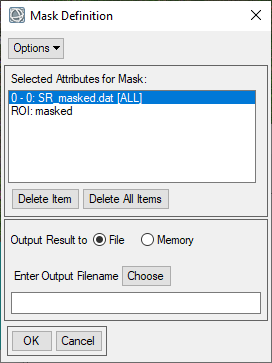
- Under Options change the mask option to "Selected Areas Off". This will produce a mask where the selected ROI(s) and no data values are masked or "off". Save the file as mymask.dat in the working folder and click OK.
- Compare the Fmask and your mask results. Select the mask that best masks all non-vegetation features for the next steps.
Calculate NDVI and Apply Mask
Normalized Difference Vegetation Index (NDVI) is designed to quickly identify vegetated areas and their condition or health. NDVI is calculated using the visible red and near-infrared bands.. Calculations of NDVI for a given pixel always result in a number that ranges from -1 to +1. Positive values indicate there is greater reflectance in the NIR as compared to visible (red). The larger the NDVI value the greater the density of healthy vegetation. Low to zero values indicate minimal vegetation. Values close to zero and negative generally correspond to impervious surfaces and water. NDVI can be calculated in ENVI using either the NDVI tool or the Spectral Indices tool or manually using the band math tool. For proper analysis data should be calibrated and corrected prior to calculating NDVI. We will use our mask created in previous steps to mask all non vegetated areas.
- From the Toolbox, select Band Algebra → Spectral Indices or type "Spectral Indices" in the Toolbox and open the Spectral Index tool. The Spectral Indices dialog appears. Select the SR_Masked.dat as your Input Data and click Mask button.
- In the Mask selection window select the best mask from previous steps (either the Fmask or mymask that you created) and click OK.
- Now we will select the desired Spectral Index from the Spectral Index list: Normalized Difference Vegetation Index (NDVI). Name your output raster "NDVI.dat" and save it in the finals folder. Click OK and by default the NDVI image should appear in the viewer.
Review the NDVI Statistics and Histogram for the Image
- Right click on the "NDVI.dat" layer in the Layer Manager and select "Change Color Table" and select one of the color tables. Applying a Color Table makes it easier to see the differences in NDVI (or any index) values.
- Another way to display and investigate data values is using the Raster Color Slice tool. Right click on the NDVI layer and select New Raster Color Slice. Select the NDVI Create raster color slice of the NDVI layer.
- Use the Chip to View option or Snipping Tool to capture an image for export of either the NDVI layer with the color table applied or the raster color slice.
A simple legend or color bar can be added to the screen under the annotations option.
Turn In - Summary Report
A Word document with:
- An overview of the data used and techniques employed.
- Compare the processing techniques and results:
- How did the radiometric calibration and dark subtraction atmospheric correction of the Level-1 data compare to the pre-processed Level-2 data? Were there differences in specific bands or certain features? Include the spectral data and graphs to back up your conclusions.
- What were the advantages/drawbacks of the different masking techniques? Which masking technique worked the best and why?
- Figure showing the NDVI image