Lab 11: Image Classification
Introduction
Classification is the process of sorting pixels into a set number of classes or categories based on the pixel values. There are two main procedures to classify pixels using a computer: unsupervised and supervised classification. Unsupervised classification is essentially computer automated. It allows you to specify parameters that the computer will use to automatically cluster or group the data. Supervised classification uses the spectral signatures obtained from training samples to classify an image. Training samples are used to collect spectral signatures from representative areas of land cover that the user designates as a certain class (e.g. water or agricultural). The computer uses the user’s specified signatures to classify all of the pixels in a scene.
In this lab we will be conducting both unsupervised and supervised classification using a new data source, imagery from the European Union's Sentinel-2 satellites. A partnership established between the European Space Agency (ESA) and the United States Geological Survey (USGS) allows for USGS storage and redistribution of data acquired by the multispectral instrument (MSI) on the European Union's Sentinel satellites. Sentinel-2A was launched on June 23rd, 2015 and Sentinel-2B followed on March 7th 2017. On September 5th 2024, a third satellite, Sentinel-2C was launched into orbit to join the other satellites. The MSI collects imagery over the Earth’s land surfaces, large islands, and inland and coastal waters with potential revisit every five days. The MSI sensor acquires 13 spectral bands with varying spatial resolution (10m, 20m, 60m). View the full list of bands and wavelengths.
About the Data: The data used in this lab is Sentinel-2 data collected in July 2025 focusing on the Lake Tahoe basin. The data has been radiometrically calibrated and atmospherically corrected and the pixels values represent the surface reflectance.
Learning Outcomes
- Learn how to conduct an unsupervised classification procedure in ENVI
- Learn how to conduct a supervised classification procedure in ENVI
- Analyze classification results, including labeling and color coding classes
- Determine the total area and percent of each class in the image
- Use Microsoft Excel to perform calculations and create tables
Set up your Workspace
First we need to set up our workspace and transfer the data for the lab.
- On the Desktop create a new folder named “Lab_11” with two subfolders, "Originals" and "Finals"
- Locate the GSP 216 Google Drive or Class Share Drive (Z:) lab data folder and navigate to the Lab 11 folder and download the ZIP file. This file contains the Sentinel-2 data. Extract the the file into your originals folder.
Opening and Stacking Sentinel-2 Data
- Start ENVI. Select File → Open and navigate to your Originals folder where you extracted your data and open the find the folder that contains the Sentinel-2 data. Open the metadata XML file that begins with "MTD_MSIL2A.xml..."
- You should now see the true color Sentinel-2 image. ENVI will automatically display the 10m resolution true color view of the scene and the other lower resolution bands (20m and 60m) files will be available in the Data Manager. Open the Data Manager
 and notice that there are many different data products included in the Sentinel-2 Level-2 bundle, visit the Sentinel-2 L2A webpage to learn what the different layers represent. Close the Data Manager when you are done reviewing the data.
 - Now we will create a Layer Stack to create one raster that includes the first 10 bands of the data in one file (the 10m and 20m resolution data). In the Toolbox select Raster Management → Build Layer Stack.
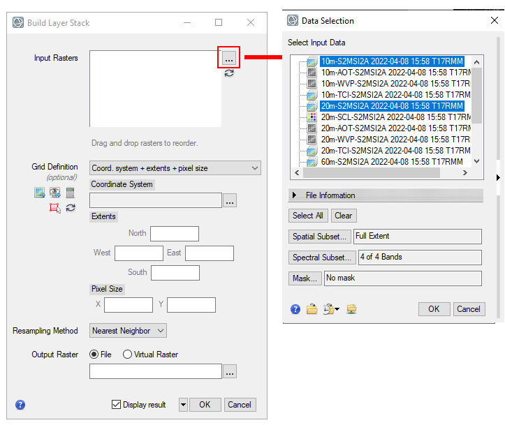
- In the Layer Stack window click to add the layer beside Input Rasters. In the Data Selection Window select the 10m-S2MSIA and 20m-S2MSIA data (hold Ctrl key to select multiple items). Click OK. The 10m data should be at the top of the list.
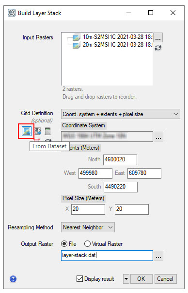
- In the main Layer Stack dialog, under Grid Definition select From Dataset. Select the 20m-S2MSIA Sentinel data file as the reference dataset. This will set the coordinate system and cell size based on this dataset. Click OK.
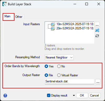
- Click back on the Main Layer Stack tab. Under Order Bands by Wavelength select Yes. The save the output raster as Sentinel_stack.dat in your finals folder. This file will contain the first 10 bands of the Sentinel-2 data, all re-sampled to 20m spatial resolution. Click OK to create and save the layer stack. Wait to the image to load and for the pyramid layers to fully load.
- Now we will create a Mask to exclude the "no data areas" from the classification process. These are areas of the raster where there is no satellite imagery. Masks can be used to only apply analysis techniques on certain areas. In the Toolbox select Raster Management → Build Raster Mask.
- In the Build Raster Mask window select the Sentinel-2 stack image (.dat) and click OK. Keep the pre-selected Selected Attribute for Mask items already populated (0). By default the mask is set to select no data value attributes, which are 0 for this dataset. In the Mask definition window select Options → Change to Selected Areas "Off" is selected under the Option drop down.
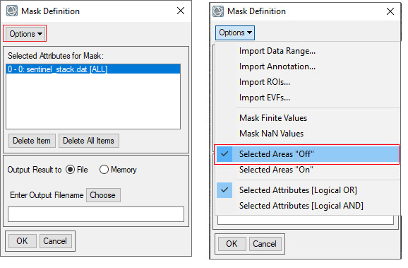
- Save your mask as nodata-mask.dat in your working folder and click OK to create the mask. The black and white binary mask (0/1) will be created for the layer (it may not appear in the view, although you can manually add or remove the mask to the view). We will use this mask in our classification workflow.
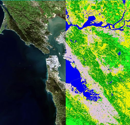
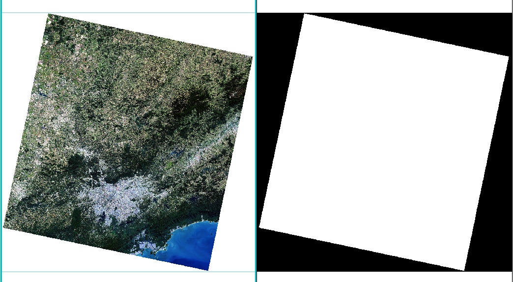 Example of a mask created for the "no data" areas of a Landsat image. The white areas (0) will be processed while the black area (1) will be masked or excluded from the classification analysis.
Unsupervised Classification
The ISODATA method for unsupervised classification starts by calculating class means evenly distributed in the data space, then iteratively clusters the remaining pixels using minimum distance techniques. Each iteration recalculates means and reclassifies pixels with respect to the new means. This process continues until the percentage of pixels that change classes during an iteration is less than the change threshold or the maximum number of iterations is reached. Start with 10 classes, although you may re-run it with more or less classes. You also can two or more combine classes after the classification. Your final classification should have between 5-6 classes (your choice based on the results and process). You will use the Combine Classes tool to combine similar classes or classes that can't be distinguished from each other.
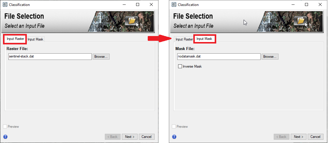
- From the Toolbox, select Classification → Classification Workflow. The File Selection panel appears. Click Browse. The File Selection dialog appears. Select the Sentinel stack file (.dat) and click OK. In the second tab select the mask layer you created in the previous step, nodatamask.dat. Then click Next to continue the workflow.
- Click Next in the File Selection dialog. The Classification Type panel appears. Select No Training Data, which will guide you through the unsupervised classification workflow steps. Click Next. The Unsupervised Classification panel appears.
- Set the Requested Number of Classes as 10. You do not need to change any settings on the Advanced tab, click Next to begin classification. The classification may take awhile. When classification is complete, the classified image loads in the view and the Cleanup panel appears.
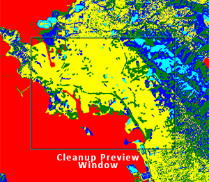
- The cleanup is an optional step, but you will use it in this exercise to determine if the classification output improves. The cleanup options are smoothing, which removes speckling, and aggregation, which removes small regions. You can check the "Preview" box to see a preview of how the cleanup will change the classification. In the Cleanup panel, keep the default settings. Click Next.
- The Export window is now open. Uncheck the "Export Classification Vector" box. Under "Export Classification Image" save the file in your "final" folder as "unsupclass.dat".
Labeling and Changing Colors of Classes
After performing an unsupervised classification you need to analyze your results. This includes determining the associated land cover type of each class, labeling the classes and changing the color on the classes. You will want to combine some of your classes, aim to have 5-6 broad land cover classes, here are recommended class ideas: Water, Developed, Forest, Agriculture and Bare Ground/Rock. You will use the Combine Classes tool to combine similar classes or classes that can't be distinguished from each other.
- The unsupervised classified image should now be in your viewer. In the Layer Manager you will see each of the classes listed separately. Right click on "Classes" and select " Hide All Classes" and then click on the image in the viewer. All of the classes are now no longer visible. We will now turn on the classes one at a time.
- In the Layer Manager click the box next to Class 1 to turn it back on. Compare the class to the satellite image to determine the land cover type. You can either turn the class on and off in the Layer Manager or use Blend, Flicker or Swipe tools to compare the class to the satellite image. You also might want to turn on the Reference Map Link to view higher resolution imagery of the area.
- Continue this process for the remaining classes. I suggest viewing one class at a time as it is easy to visually compare. Write down the class number and corresponding land cover type for all classes. We will update the names and colors in the next steps. If some classes are similar, you may want to label as "Vegetation1", "Vegetation2" for example and combine these classes (see step 31). Note that the class names must be unique (i.e. two classes can't both be named "forest". Label the classes to the best of your ability. You can combine similar classes in step 20.
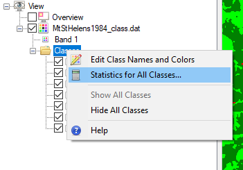
- Expand the classification file in the Layer Manager and right click on the "Classes" and select and select Edit Class Names and Colors.
- The Class Name and Color Editing window is now open. Here you can change the names and colors associate with each class. Start with Class 1 by clicking on "Class 1" in the list. Under Class Name update the name to the land cover type (for example "Water" or "Developed").
- Select the drop down Color, and select an appropriate color for the class. I suggest using an intuitive color (i.e. blue for water).
- Repeat this for all classes (you can leave unclassified and masked pixels as-is). Once you are done click OK. The classes should now be renamed and have new colors.
- Use the Combine Classes tool (Classification → Post Classification →Combine Classes) to group similar classes together. For more information see: https://www.nv5geospatialsoftware.com/docs/CombiningClasses.html. Save your new classification file in your finals folder.
- Take a screenshot or use the Chip to View tool to save unsupervised classified image (turn off all other layers). Include this as a figure in your report.
Viewing Statistics for Unsupervised Classification
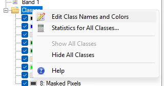
- Expand the re-named and cleaned up classification file in the Layer Manager and right click on the "Classes" and select "Statistics for All Classes". In the Data Selection Window selected the classified image you want to view the statistics for and click OK.
- Highlight all of the class names (leave out unclassified and masked) and the pixel count column and select the Copy to Clipboard option.
- Start Microsoft Excel or Google Sheets and open up a blank workbook. Paste your classification statistics into the sheet. Add a column for color. Change the color of each cells to match the color of the classification output. You can do this by right clicking on the cell and selecting Format Cells → Fill or select Fill Color
 from the toolbar. This will help you table also serve as a legend for the classified image.
 - Calculate the area in Hectares or Acres (10,000 m2 equals 1 Hectare, 4046.86 m2 equals 1 acre) for each of the classes. The area of a class can be determined by multiplying the pixel count for each class by the area of one pixel. This can be done quickly in Excel by using formulas. See video at start of section.
- In the area column after the last row with data, we will calculate the total area. In the cell type =sum( and then highlight the the area of all of the classes and hit enter. This will automatically sum up all of the data you have selected and provide the total area classified.
- To the left of the area column start another column to calculate the percent area of each of the classes. In the top cell type = and then select the adjacent cell with the area and type / and then select the cell with the total area. Edit the formula to add a $ in front of the cell referencing the total area (for example $F$6), this will make it an "Absolute Reference", meaning even if you copy the formula, the same cell will always be referenced. Copy the formula to the other cells by dragging the corner of the cell down. Change the cell data type to percent.
- Save your Excel spreadsheet in your "Final" folder, you will need this table for your final report. The table will provide quantitative data and also serve as a legend for your classified image.
Supervised Classification
Supervised classification clusters pixels in a dataset into classes based on user-defined training data. The training data can come from an imported ROI file, or from regions you create on the image. The training data must be defined before you can continue in the supervised classification workflow. In this lab we will define out training data first and then import the training data ROIs into the classification workflow. We will use the satellite imagery to visual identify appropriate training areas.
- Based on the results of the unsupervised classification, identify 4-6 classes to collect training data for. Right click on the Sentinel-2 stack file and select New Region of Interest. We will create a separate ROI for each of the classes we want in our classification. Each ROI should have multiple polygons to collect training data.
- In the ROI Tool window change the ROI Name from the default to "Water" and change the color as appropriate. The color selected will be the color assigned to this class once the classification process is complete.
- Training classes are selected by creating selecting several representative polygons or sample areas for each class. Locate a region that is water in the image. Draw a polygon to select the area as a training area that represent water. Repeat this process, creating a total a minimum of five polygons that represent water. Try to sample areas that are in different regions of the image to capture a range of water types.
- Click the New ROI icon in the ROI Tool Window. This will be the ROI for the seconds class. Repeat steps for the next class (use the same classes you identified in the unsupervised classification). You may want to research the area, use the reference map and/or other maps like Google Maps to help identify appropriate training data.
- Repeat steps above to create ROIs and collect training data for all of the classes. You should have between 4-6 classes total. Once all of the training data has been collected, in the ROI Tool window select File →Save As. Select the all of the training data ROIs and save the file in the Final folder.
- From the Toolbox, select Classification → Classification Workflow. The File Selection panel appears. Click Browse. The File Selection dialog appears. Select the Stacked Sentinel-2 image and click OK.
- Click Next in the File Selection dialog. The Classification Type panel appears. Select "Use Training Data" and click Next. This will start the Supervised Classification workflow. If prompted for ROI visualization layer, select the masked file. This will only show the Sentinel-2 areas that are within the mask.
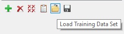
- The Define Training Data will open. All of the ROIs should be listed in the Training Data window. If your ROI Mask is listed in the training data window, remove it by clicking the red "X". If the training data ROIs don't automatically populate, you can click the "Load Training Data Set" folder icon and find the training data file. ENVI can import training data stored as either XML files or Shapefiles.
- Under the Algorithm tab, select Spectral Angle Mapper from the drop-down list provided. Next you will preview the classification results, based on the training data you provided. Enable the Preview option to open a Preview Window that shows the classification result using the training data that you created. Change the algorithm type to see the impact on the classification results. If ENVI crashes at this point you will have to restart the classification workflow. As long as the training sites have been saved you can simply import the existing sites by clicking the "Open" icon in the training sites window. The Preview is optional therefore don't use it if it leads to crashing.
- Click Next. When supervised classification is complete, the classified image loads in the Image window, and the Cleanup panel appears. In the Cleanup panel, keep the default settings. Click Next.
- The Export window is now open. Uncheck the "Export Classification Vector" box but keep the "Export Classification Image" box checked. Under "Export Classification Image" save the file in your "Final" folder as "supervisedclass.dat".
- Click "Finish" to complete the classification and save the classification files.
- The supervised classified image should now be in your viewer. Visually compare the supervised and unsupervised classification by turning the layers on/off or using the Blend, Flicker and Swipe tools. Note which classes appear the same in the two images and which classes differ.
- Take a screenshot or use the Chip to View tool to save supervised classified image (turn off all other layers).
Viewing and Saving the Statistics for Supervised Classification
- Repeat steps 26-31 for the Supervised Classification image.
Lab Report (Upload to Canvas)
Prepare a lab report that discusses the results of the unsupervised and supervised classification. Your report should include all of the figures and classification results in tables and discuss the results in a Results/Discussion section. In your results include a table with the total area in hectares or acres and percent area of each class for both the unsupervised and supervised classification. Make sure your report includes the following items:
- Name, Date and Title
- Results and Discussion
- Figures (2): The Unsupervised Classification Image and the Supervised Classification Image. You may also want to include an figure showing the satellite images, but this is optional.
- Tables (2): Tables showing the total area in hectares or acres and percent area of each class for both the unsupervised and supervised classification.
- Results and Discussion including the following items:
- Compare the supervised classification to the unsupervised classification results for the data, how did the results differ?
- For each of the the classifications (unsupervised and supervised) which land cover features (i.e. water, developed etc.) appeared to be most accurately classified and which incorrectly classified?
- What are the advantages/disadvantages of each of the classification procedures?