Lab 10: Raster Analysis
Introduction

In this lab, we will conduct a spatial analysis using remotely sensed data. We will use a recent Landsat 8/9 Level 2 Surface Reflectance Data of the Mt Shasta region (acquired in April 3rd 2026), a Digital Elevation Model (DEM) and a watershed boundary of the region to conduct a raster based spatial analysis. The purpose of this analysis is to locate, quantify and analyze areas of snow cover within the seven watersheds that encompass Mt Shasta. The satellite data used is Landsat Collection 2 Level-2 Surface Reflectance Data. This Landsat data has been radiometrically calibrated and atmospherically corrected and the pixel values represent surface reflectance percentage.
Learning Outcomes
- Work with Landsat Level-2 Surface Reflectance Data.
- Mosaic data in ENVI
- Re-project spatial data in ENVI
- Use the Band Ratio Tool and Raster Color Slice to isolate features in ENVI
- Download and process Digital Elevation Models (DEMs)
- Use the Spatial Analyst tools in ArcGIS Pro
- Use the Raster Calculator tool in ArcGIS Pro to conduct raster analysis
Set up your Workspace
First, we need to set up our workspace and transfer the data for the lab.
- On the Desktop create a new folder named “Lab_10”.
- Within the folder named “Lab_10”, create three subfolders as below:
- Originals
- Working
- Final
- Locate the GSP 216 Google Drive lab data folder and locate the file "Lab10 data" Zip file and download the file. Extract the ZIP file data into your "Originals” folder. There should be three files, two folder containing shapefiles and a Landsat "tarball" (.tar) file. Uncompress the Landsat file in your original folder. Now all of the files should be uncompressed and ready to use.
Working with Landsat Surface Reflectance Data : Save and Subset Images and Calculate Ratio Index
- Start “ENVI ” and Select File → Open and navigate to your Lab 10 Originals folder where you extracted your data and find the folder that contains the Landsat data and open the metadata text file (..._mtl.txt) associated with the data. Note that the Open As option does not work with Landsat Level-2 data, the metadata text file (..._mtl.txt) can also be dragged and dropped into the ENVI viewer to open the Level-2 data.
- Open the Shasta Watersheds Shapefile "shasta_watersheds.shp ". This data was extracted from the National Watershed Boundary Dataset (WBD) and includes the boundaries of the seven watersheds that encompass Mt. Shasta.
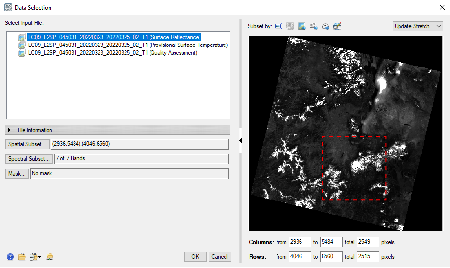
- Before we can process the data, we will save and subset the surface reflectance data. This is necessary when working with Level-2 data. From the main menu select File → Save As.. (ENVI...).
Select the file "Surface Reflectance" data from the list, click Spatial Subset. Select the Subset by Vector icon and select the shasta watershed shapefile and then save the file as MtShasta.dat in your Finals folder and click OK.
Snow has high reflectance in the visible and low reflectance in the shortwave infrared. There are several different tools that can be used to enhance and extract spectral differences. We will test out a spectral index, band ratio and band difference to compare the reflectance of two bands.
- Open the Data Manager and remove all the original Landsat files and leave the MtShasta.dat and Shasta_Watersheds shapefile. Change the band combinations of the MtShasta.dat image to Red - SWIR, Green - NIR, Blue - Red or set to Shortwave IR predefined. This will make the snow appear bright blue and easier to differentiate from other land cover.
- Use the spectral profile tool to investigate the reflectance curve of some of the snow areas. Make note of where in the spectrum the highest and lowest reflectance, these are the bands that should be used when selecting appropriate spectral enhancements. We will try several different methods and select the best results for differentiating snow cover.
Normalized Difference Snow Index (NDSI)
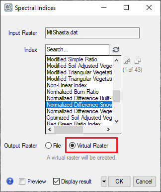
- From the Toolbox, select Band Algebra → Spectral Indices or type "Spectral Indices" in the Toolbox and open the Spectral Index tool. The Spectral Indices dialog appears. Select the MtShasta.dat is your Input Data and click OK. In the next window select the Normalized Difference Snow Index from the list. Instead of saving the output raster as a file select Virtual Raster. This will save the file in temporary memory allowing us to review the results without permanently saving the file.
- Check out the results of the NDSI calculation. Higher values generally indicate snow, although a positive NDSI value is indicative of any material that has lower reflectance in the SWIR than in the Green wavelengths. Compare the results of the NDSI to the false color composite image. Note that while theoretically NDSI values should range from -1 to 1 values outside this range can occur if there are negative values in the original data. This can occur in some atmospherically corrected imagery and sometimes additional processing is required.
Calculate the Band Ratio
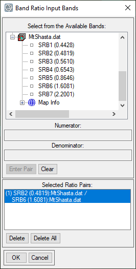
- In the toolbox select Band Algebra → Band Ratio. For the MtShasta.dat file, select SRB2 (0.4819) which corresponds to the blue wavelength as the Numerator and SRB6 (1.6081) the SWIR1 as the Denominator and click Enter Pair.
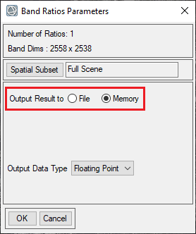
- In the next window save the output results to Memory rather than file. This will create another virtual file that we can use to view the results. Keep the rest of the defaults and click OK.
- Compare the results of the band ratio to the false color composite and snow cover. Larger values indicate higher ratio between the visible and SWIR.
Calculate the Band Difference
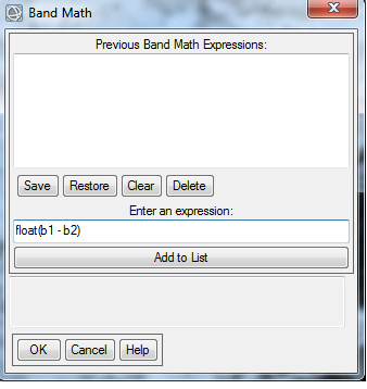
- From the Toolbox, select Band Algebra → Band Math or type "Band Math" in the Toolbox and open the Band Math tool. The Band Math window will open. Enter the following expression: float(b1 - b2) and click OK. This will calculate the difference between any two data sets (the same expression was used to calculate dNBR).
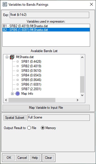
- The Variable to Bands Pairings window will open, this is where you will we tell ENVI which bands or data to use for the variables (b1 & b2). For B1 select SRB2 (0.4819) which corresponds to the blue and select SRB6 (1.6081) as B2, saving the output results to Memory again rather than to a file.
- Compare the results of the band difference to the false color composite and snow cover. A large positive value in the band difference is indicative of snow. This layer should give the a high degree of contrast between snow and other land cover. Compare all three of the images (NDSI, Band Ratio and Band Difference) and select the image that best differentiates snow from all other land cover types.
- Open the data manager and remove of the files except the spectral enhancement file you selected in the previous step (NDSI or Band Ratio or Band Difference), the subsetted Mt Shasta Landsat image and the watershed shapefile.
Sample Areas of Known Snow Cover
To better isolate the snow covered areas in the image we will use reference data. These are locations with known snow cover. This will help us decide what values represent snow and to select an appropriate threshold.
- In the main toolbar, open the file "Shasta_Snowcourses.shp" from the originals folder. This shapefile contains points with the locations of five Snow Course stations that are sampled for snow depth and water content by the California Department of Water Resources.
- Right click on the shapefile layer and select View/Edit Attributes. This will open the attribute table associated with the shapefile. In the Attribute Viewer window select Options >Add Column. This will allow us to add a new column (or attribute field).
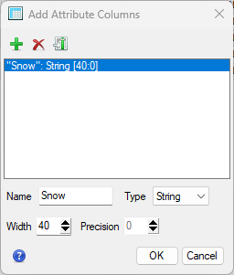
- In the Add Attribute Columns Window, name the new attribute Snow and set the type to String and press OK.
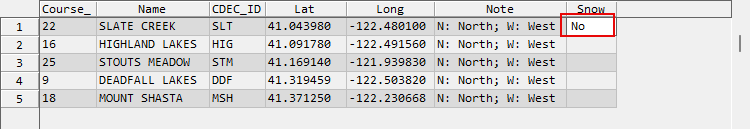
- Now you should see a column labeled "Snow". In this column we will add data indicating whether or not snow was measured at the location in the field. Visit https://cdec.water.ca.gov/reportapp/javareports?name=COURSES and search for the snow course measurements from April 2026, see help forum if you are having issues with the website. Search for the names of the five snow courses included in the shapefile (e.g. Slate Creek) and note whether or not snow was observed at the most recent measurement. A Depth value of "0" means no snow was present, any other number indicates some level of snow. Update the Snow attribute field by for each site by double-clicking in the field. Update to either "Yes" for snow or "No" for no snow measured. Click File > Save in the Attribute Viewer window when you are done.
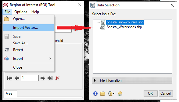
- In the Layer Manager right click on the spectral enhancement file you choose in step 15 and select New Region of Interest. In the ROI Tool window select File → Import Vector. In the Data Selection window select the "Shasta_snowcourses.shp" file and OK.
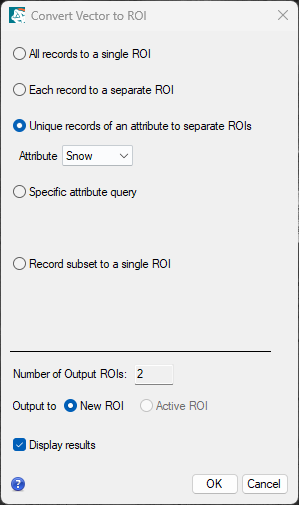
- In the Convert Vector to ROI window and select the "Unique records of an attribute to separate ROIs" and select Snow as the attribute and click OK. This will create two ROIs, one with sites that have snow and one with site without snow. Select the spectral layer as the Visualization Layer if given an option.
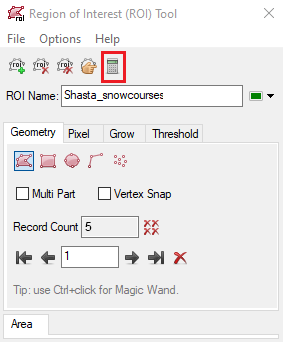
- Now there are two ROIs, one that represent areas that have snow on the ground and one for areas without Snow. In the Layer Manager, right click on the Regions of Interest folder and select Statistics for All ROIs. This will generate summary statistics for both ROIs (Snow and No Snow).
- Write down the minimum, mean and max values for both the Snow and No Snow data, we will use as this data to help set the snow threshold (i.e. areas with a value greater than the minimum snow value should be snow and areas with values lower than the minimum value are not snow covered). Close the ROI window when you are done.
We will use the Raster Color slice to create a single class that isolates the snow in the image by selecting a range of values.
- In the Toolbox navigate to Classification → Raster Color Slices. Select the spectral enhancement file as the input and click OK.
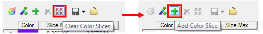
- Delete all of the existing slices by clicking Clear Color Slicing. Then create one new Color Slice by clicking Add Color Slice. We will only be creating one class which represents snow.
- Use the value from step 20 as the slice Min and keep the Slice Max as the default value (should be the maximum value found in the image).
 Zoom in on your image and turn the Raster Color Slice layer on and off to preview your selection. Make adjustments by either changing the Slice Min value or by manually dragging the bar on the histogram to make adjustments to the range of the class/slice based on visual analysis. Try to make sure your selection includes all of the snow and no other features.
![]()
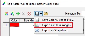
- In the Raster Color Slice window export the data by clicking the save icon and selecting Export as Class Image. Save the file as snow.dat in your Working folder.
- The last step is to mask the snow layer you just created to the boundaries of the watersheds. From the main menu select File → Save As (ENVI..) and select the snow.dat file as the input file. Click the Mask option and select the Shasta Watershed shapefile. Save the file as "shasta_snow.dat" in your Final folder.
Download and Process Digital Elevation Models
- Go to The National Map download interface: https://apps.nationalmap.gov/downloader/. A variety of data can be downloaded from the National Map interface. We will be looking for Digital Elevation Model data. You can also download Hydrography and Boundary as well as a variety of other data from the National Map.
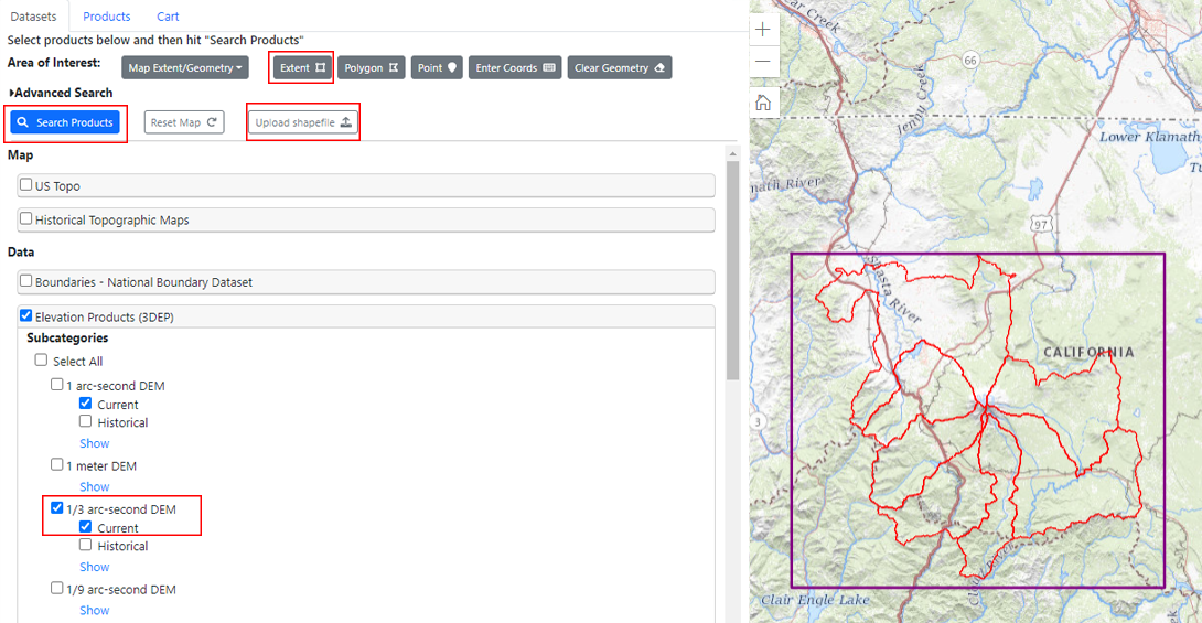
- Data can be selected by Map Extent, Polygons or for specific coordinates. Shapefiles can also be uploaded for visualization purposes and then you may also use the polygon or extent tool to draw a rough outline around the shapefile of interest. Click on the Upload Shapefile button and select the zipped Shasta Watersheds shapefile (Shasta_Watersheds.zip). You should now see the Mt. Shasta watershed boundaries on the map.
- Click the extent button to draw a bounding box around the shapefile on the map. This will limit the data search to the Mt. Shasta watershed boundaries.
- Under Data on the right hand side check Elevation Products and select ⅓ arcsecond DEM. ⅓ arcsecond corresponds to approximately 10 meter spatial resolution. Keep the Data Extent as 1 x 1 degree and the File Format as GeoTIFF, IMG. Click the blue Search Products icon to search for data.
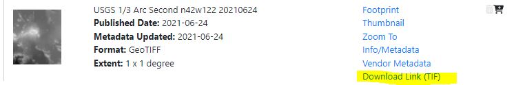
- In the Available Products window there should be at least two datasets, one directly cover Mt Shasta and one to the east, the corresponding map index names are: Weed E and Alturas W. Click the Footprint to make sure they cover the area. Download the most current GeoTIFF dataset for each location: USGS 1/3 arc-second n42w123 1 x 1 degree and USGS 1/3 arc-second n42w122 1 x 1 degree These files cover the area of the Mt. Shasta Watersheds.
- Find the datasets in your downloads folder and move them to your Originals folder. The DEM files will be .tif (GeoTIFF) files.
- We want to mosaic the two DEMs together into one seamless file for analysis. In the ENVI Toolbox select Mosaicking → Quick Mosaic. Use the Quick Mosaic tool to create a virtual mosaic of georeferenced rasters and to mosaic data that doesn't need advanced processing. For advanced mosaicking methods such as color balancing and edge feathering, use the Seamless Mosaic workflow.
- Click the "+" icon to add the scenes be mosaicked. If you haven't added the DEMs to ENVI yet, click the folder icon to locate and open the DEM files. Select your two DEM tif files from your originals folder and click OK (use the shift button to select more than one file).
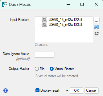
- Leave the Data Ignore Values blank and select Virtual Raster as the Output Raster. This will create a temporary mosaicked raster dataset, which we will use for further processing. Make sure Display Result is also checked and click OK to run the tool.
- When the new mosaicked DEM appears it will say [RE-PROJECTED], which indicates this file has a different spatial reference system than the other files. Therefore we will need to re-project the DEM raster. We also want the pixels of the DEM to be the same size and match up with the Landsat derived snow layer (30m). The Regrid Raster tool in ENVI is one way to accomplish this task. In the Toolbox, select Raster Management.
The Regrid Raster tool allows a user to re-sampled and re-project raster files to a specified spatial grid, which includes a specific coordinate system and pixel sizes. Making sure all data have the same coordinate system and pixel size is necessary for many raster analysis techniques.
- In the Regrid Raster tool window select the mosaic DEM as the input raster. Under Grid Definition leave the default option (Coord system + extents + pixel size) and click the From Dataset icon
 . Select the shasta.dat multispectral file as the reference dataset. This will set the coordinate system and cell size based on this dataset. Click OK. The window should now update showing the coordinate system, extent and pixel size from the Landsat data.
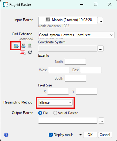
- Change the Resampling Method to Bilinear and save the Output Raster file as DEM_UTM.dat in your finals folder and click OK to run the tool. When the process is finished a the re-projected and re-sampled DEM should appear the Layer Manager, this time without saying [REPROJECTED]. Check to make sure the following files are in your finals folder: Shasta.dat (subsetted Landsat image), Shasta_snow.dat and DEM_UTM.dat. You may close ENVI when you are done.
Raster Spatial Analysis in ArcGIS
We will use the Snow file, Watershed Boundary shapefile and the Digital Elevation Models (DEMs) to analyze the extent and area of the snow. The first step will be to determine the amount of snow in acres within the seven Mt. Shasta Watersheds. Then we will conduct a more in-depth analysis including looking at the snow cover by aspect (slope direction) and elevation. Before using many of these tools you will need to make sure the Spatial Analyst extension in enabled in ArcGIS.
Determining Area of Snow Layer
- Start ArcGIS Pro and create a new map project in your lab finals folder. Connect to your Lab 10 folder in the Catalog to make it easier to access and manage data. Move the Shasta watersheds shapefile from the Originals to the Finals folder.
- In the Geoprocessing Pane search for or select Toolboxes →Data Management → Raster → Raster Properties →Build Raster Attribute Table. Select the Shasta Snow layer (shasta_snow.dat) snow layer from your finals folder and click Run. This will add an attribute table to the files that include the class value (1, indicating snow) and the number of pixels in each class, this file should be added to the map after the process is complete. Note that in order for the Build Raster Attribute Table function to work properly it must be done before adding the data to the map.
- Add the Shasta watersheds shapefile, the satellite imagery (MtShasta.dat) and the UTM DEM file from your map.
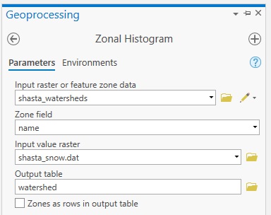
- Make sure the Spatial Analyst extension is enable (see below box). In the Geoprocessing pane search for Zonal Histogram or select Spatial Analyst Tools → Zonal → Zonal Histogram. The Zonal Histogram will calculate the number of pixels (count or frequency) in one dataset within classes or regions of another dataset.
- In the Input Raster or Feature zone select select the Shasta watershed shapefile. In the Zone Field select Name. This will summarize the number of snow pixel by the watershed name. In the input value raster select the Shasta Snow layer and save the table as wateshed_snow in your final folder. This table will summarize the number of snow pixels within each watershed.
- The table will automatically be added to your Table of Contents. Right click on the file and select open. The table shows the number of snow pixels in each of the seven watershed boundaries. We will use this information to calculate the area of snow in acres. Select the row with the data and copy the data and paste into Excel.
- Check the spatial resolution on the Snow layer by right clicking, selecting Properties and writing down the Pixel/Cell Size. Use the below guide to calculate the area of snow in each watershed in acres and the total area within all seven watersheds.
Example: Calculating Area of Raster Class
First determine the spatial resolution of the raster and the number of pixel in the class or category
Total Area of class in square meters= spatial resolution2 x pixel count for class
Note that 1 acre = 4046.86 m2
Create an Aspect Raster
The aspect of terrain refers to the direction it’s facing and is computed in degrees from due north. Aspect relates to the amount of sun exposure, in the northern hemisphere a north-facing slope faces away from the sun and therefore is generally cooler and wetter than a south-facing slope. The aspect of a slope can have significant influence on its micro-climate and vegetation. Given this influence on vegetation, aspect is frequently used in raster analysis. Aspect is always given as a direction in degrees, for example a North facing slope the aspect would be between 0-22.5 degrees.
- From Geoprocessing Toolbox, select Spatial Analysis Tools → Surface → Aspect.
- Set the "Input Raster" to be your Elevation layer (DEM). Save the "Output" raster to your working folder and name it "Aspect.tif”. Leave the default method as PLANAR and click Run to create the file.
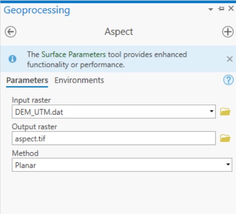
- You will now see your Aspect raster in your window. The Aspect identifies the downslope direction of the maximum rate of change in value from each cell to its neighbors . Aspect can be thought of as the slope direction. The values of the output raster are the compass direction of the aspect, a color coded classified symbology is used to display the degrees as directions.
Aspect in ArcGIS
 By default aspect files are usually generated with a color coded scheme where the degree values are grouped into directions (North, Southeast etc). You can also add the Colormap function to display the dataset using the color map renderer or a specified color scheme.
Create a Hillshade Raster
Hillshades are common background used in maps. A hillshade is a 3D representation of a surface using the sun's relative position to provide shading and depth to the image. A hillshade is a raster that essentially appears to be a photo from above the sea, shaded by the sun. Hillshades are not used for analysis but provide nice backgrounds for maps and data.
- Navigate to the Geoprocessing → Spatial Analysis Tools → Surface → Hillshade.
- In the Hillshade dialog box select the elevation layer (DEM)as the input raster file. Save the output raster in your Finals folder as "hillshade.tif”. Keep all of the default settings. Click OK to create the hillshade raster. You should now see the hillshade file in your viewer.
- Move the hillshade to the bottom of your layers for now. We will need it to create our map later.
Analyze Snow Cover by Aspect
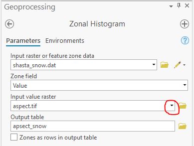
- Run the Zonal Histogram tool to determine the number of snow pixels in each aspect class (North, Northeast etc). For the Input Zone, select the snow layer (shasta_snow.dat) and the aspect layer as the Input Value Raster. When selecting the aspect layer use the dropdown arrow to select the file. This will select the file with the classified symbology (North, East etc). Save the table as "aspect_snow" in your finals folder.
- Use the same process as step 40 to calculate the area in acres of snow for each of the nine aspect classes.
Determine Snow Cover Elevation Range
Zonal Statistics by Table: This tool summarizes the values of a raster within the zones of another dataset (either a raster or shapefile) and reports the results to a table. The stats include the mean,minimum, maximum values etc.
- Go to the Geoprocessing Toolbox , select Spatial Analyst Tools → Zonal → Zonal Statistics as Table. Select the Snow layer (shasta_snow.dat) as the Input Zone (leave the file as Value) and Select the Input Value Raster as the elevation (DEM). This will provided statistics about the elevation data within the area where snow is present. Save the output table as elevation_stats in your final folder.
- Open the table and copy the statistics into your Excel spreadsheet. Note the minimum and maximum elevation values. This tells us the minimum and maximum elevation that snow was found at in the image.
Analyze Snow Cover by Elevation Range
We want to create an output raster that shows areas that have snow by elevation range. We will use the Raster Calculator to accomplish this.
- We want to divide up the elevation into three elevation classes, low elevation snow, mid and high elevation. The elevation ranges will be:
- Low Elevation: 0-1500 (less than 1500m)
- Mid Elevation: 1500-2999 (more than 1500, less than 3000m)
- High Elevation: 3000-4500 (greater than 3000m)
- Start the Raster Calculator by going to the Geoprocessing , select Spatial Analyst Tools → Map Algebra → Raster Calculator.
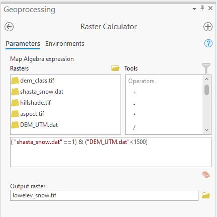
- We want a raster that will display all of the areas that have snow and that are in the low elevation range (as determined above). Double-click on the snow file to have it added to the equation box, click on "==" and then type 1. This will select for area that have snow (values of 1). Be sure to also add parentheses ( ) around your expression. Now click the “&” operator. Double-click on the elevation layer and then click on "<" and then type 1500 (the desired elevation value), again be sure to also add parentheses ( ) around your expression. Save the output raster as “lowelev_snow.tif” in your Lab 10 “Final” folder. Your dialog window should look like the one below.
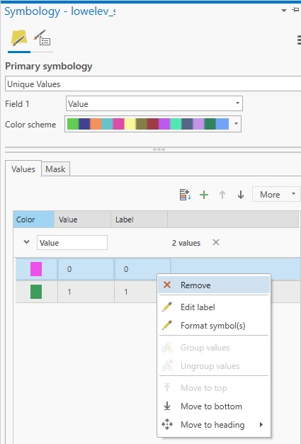
- The raster file should have automatically been added to your Table of Contents. Remove 0 class from display by going into the Symbology and removing the "0" class. The areas show in color (1) meet our criteria, i.e. low elevation snow cover. You can also label the "1" class as Low Elevation Snow.
- Repeat Raster Calculator process to create a raster layers for the remaining two elevation classes, mid elevation snow and high elevation snow. Keep the first first of the expression the same ( "shasta_snow.dat" ==1)
but adjust the elevation criteria using the following guidelines:
- Mid Elevation Range: Greater than or equal to 1500 and less than 3000. Note that each you will need to put () parentheses around each expression component and each elevation criteria needs to be a
evaluated seperately, for example to find to find elevations between 1500 and 3000 meters: ("DEM" >=1500) & ("DEM" <3000)
- High Elevation Range: Greater than or equal to 3000
- For each of the three analyses, right click on the layer and select Open Attribute Table. Record the number of pixels that are classified as snow (1) in each of the analyses. You will also need to verify the spatial resolution of the data. This can be done by right clicking on the file and selecting properties. In the Layer Properties window click the Source tab and note the spatial resolution (cell size).
- Use the above information to calculate the area of snow in acres for each of the elevation ranges. You will use this information to create a bar graph in Excel or Google Sheets showing the area of snow in each elevation class.
Create a Map Displaying Snow Cover by Elevation Range
- Re-arrange the layers so that the three snow elevation layers are on-top, with the layer hillshade uder the layer. You can remove or hide all of the other layers on the map. Remove the default ESRI basemaps and hillshade as well.
- Select the low elevation snow layer in the Content and click on the Raster Layer tab in the main toolbar. Under “Transparency” change it to “50%”. Change the transparency for all three of the snow layers to 50% as well. You may adjust the transparency % as you see fit.
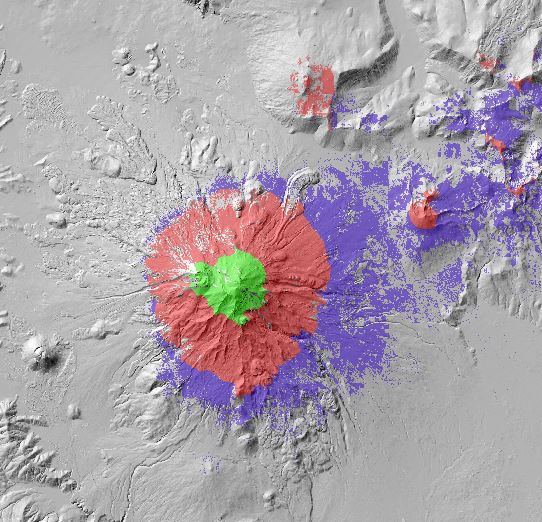
This is a example figure for 2017 data, your final image will look different.
- Create a map layout that include a title, north arrow, scale and legend. The legend should include the three snow elevation classes labeled with the class name. You may focus your map on Mt Shasta if you like or include the entire study area.
- Save your map and export the map as JPG. Back up your final folder when you are done. Make sure had all of the data needed to complete the questions. Use Excel/Google Sheets to perform the calculations and to create tables and graphs for the report. A tables and graphs should be professionally formatted and easy to read.
Lab (Upload to Canvas)
Present the results of your raster analysis in a document. You do not need to include an introduction or other components of a lab report, but your results should be articulated in complete sentences with professional-looking tables and figures.
Include a short written summary of the following results that includes the following information:
- How many acres of snow were within the Shasta Watershed boundary (all seven watersheds)?
- Which watershed had the least amount of snow cover by area? Which had the most amount of snow?
- What was the lowest elevation at which the snow was found?
Figures and Tables: All figures and tables should be labeled (e.g., Figure 1) with appropriate captions.
Figure 1: Mt Shasta Watershed Snow Map
- Snow coverage results for the three elevation classes (low, mid and high) over-top the hillshade
- Cartographic Elements: Title (optional since a caption with be included), Legend with Class names, Scale, North Arrow, Data sources and Map author.
Tables - Should be professionally formatted and easy to interpret
- Acres of snow within each of the seven watersheds (by name)
- The snow area in acres by elevation class:
- Low Elevation
- Mid Elevation
- High Elevation
Figure 2 - Graph
- A bar graph or pie chart showing the area of snow in acres by aspect (e.g., North, Northeast, etc.) or the percent (pie chart).
