Lab 7: Working with Publicly Available Lidar in ArcGIS Pro

Introduction

Lidar point cloud datasets that can be managed, visualized, analyzed, and shared using ArcGIS. ArcGIS Pro supports lidar data provided as LAS format (industry standard) and the ESRI specific Optimized LAS (.ZLAS) format. There are a variety of tools available to process, view and edit lidar data in ArcGIS Pro. One of the most efficient ways to utilize Use lidar as a LAS dataset The LAS dataset provides fast access to large volumes of lidar and surface data without the need for data conversion or importing.

About the Data
This data is lidar points clouds data available through the USGS 3D Elevation Program through the National Map. The area of interest is Cal Poly Humboldt owned Goukdi’n- Jacoby Creek Forest.

Create ArcGIS Project and Decompress LAZ Files

1. On your local workstation, make a folder for your work with the following subfolders: LAZ, LAS, Rasters. Copy the data from Z: or Google Drive to your local workstation. Then, place the LAZ files into the LAZ folder you created. Finally, make a folder for your work. Transfer the Shapefile of Forest Boundary to your main folder and unzip.
2. Start ArcGIS Pro and save your project as JCF Lidar (or something similar) in your folder. In the Catalog pane, add your lab folder as a folder connection to the project.
3. We need to confirm the spatial reference system (aka coordinate system) for the data before we start. This information is typically found in the metadata file. In the Catalog pane, locate the metadata file (XML) in the LAZ folder, right-click on it, and select View Metadata. 
4. In the metadata window, you will likely see a message that ArcGIS Pro can't read the FGDC metadata. Click the View Content link to open the metadata file in a new window. Search for both the Vertical (Z or height, vertdef tag) and Horizontal Coordinate System (XY, horizsys tag). Write this information down or leave the window open for reference. We will need this information for the next step. 
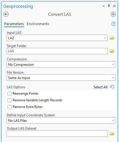
5. The compressed LAZ files need to be uncompressed into the LAS format before they can be viewed or analyzed in ArcGIS. In the Geoprocessing Pane, locate or search for the Convert LAS Tool (Conversion Tools > Point Cloud> Convert LAS) and launch the tool.
6. The Convert LAS tools allows the user Converts .las, .zlas, and .laz files between different LAS compression methods and file versions. In this tool you can select a single LAZ/LAS file or an entire folder to compress/decompress. To convert all LAZ files, select your "LAZ" folder as the Input LAS. This will convert all applicable files located in this folder. Make sure your LAZ files are in the folder (and not in a subfolder). Select the "LAS" folder as the Target Folder. Compression should be set to No Compression (extracts or decompresses files) .
7. In the Define Input Coordinate System select LAS Files with No Spatial References. Set the spatial references as noted from the metadata. You will need to specify both an XY (horizontal) and Z (vertical) coordinate system. For lidar files, the horizontal coordinate system must be a projected coordinate system! The units for the coordinate systems should be linear (either meters or feet), check before proceeding. Save the output LAS Dataset as JCFLidar.lasd (or something similar) and click Run to convert the files and create the LAS dataset.s
8. Once the tool has finished running check the LAS folder to make sure that there are 11 LAS files in the folder. The LAS Dataset should automatically be added to your map. By default you will only see the footprint of each individual LAS file.

Creating and Viewing LAS Dataset

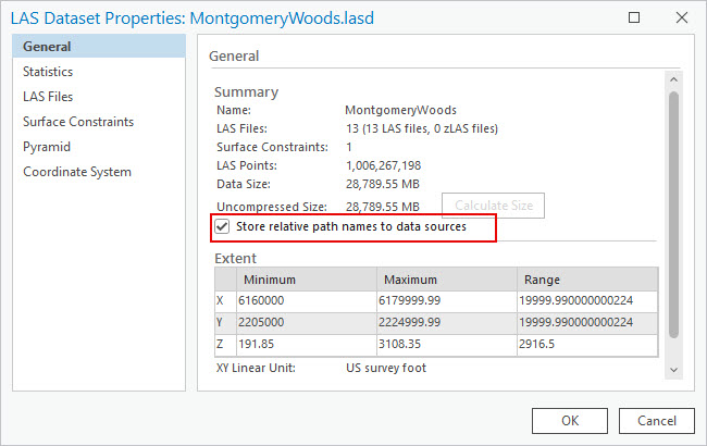
8. In the Catalog Pane right click on the LAS files and select properties. Check the Coordinate System information.  Make note of the linear units and the Horizontal and Vertical Coordinate System. Under the General tab check the Store relative path names to data sources box. The total number of points and number of LAS files are noted on this tab.
9. Click on the LAS Files tab. You will see the file names and basic statistics for all of the LAS files that make up the LAS Dataset.  Make note of the point spacing for all of the files and calculate the average point spacing the dataset. Tip: You can select and copy all of the of LAS file information from this window and paste it into a spreadsheet.
10. Click on the Statistics option. By default the statistics should be calculated, if not click the Calculate button to produce the statistics for this LAS dataset from the LAS files you added.
11. Review and find the following information: How many different classification categories are there, how many return classes are there? How many points total? You will need this information for your lab turn in. Close the LAS Dataset Properties when you are done.
12. Now add the shapefile showing the boundary of the forest . By default you will only see the outline of the footprints of the LAS files that make up the dataset. There are too many points to draw. If you zoom to ~1:2,000 scale you should see the points.
13. Zoom back out so only the outlines of the LAS tiles are visible. Click on one the LAS files. The pop-up will display information for the selected file. You can view general information in the pop-up, including the point count, spacing and density, as well as more detailed information on the return values and classification codes that are available for the selected LAS file.
14. Zoom in until you see individual points. Click on one of the points and look at the attributes. Check the time GPS time, use the internet to try and determine what time and date the lidar data was collected.
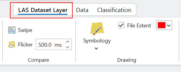
15. Now we can check out different ways to visualize the data points in 2D. Click on the .lasd file in the contents pane to select it as the active layer. Now there will be a LAS Dataset Layer tab in the main ribbon. Click the LAS Dataset tab. This controls the appearance and how the LAS data is displayed.
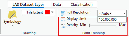
16. First change the Point Thinning options. This allows some control over how many points can be rendered on the map. The density allows for more or less points. The maximum Display Limits is 100,000,000. Try increasing and decreasing the display limits to see the difference.
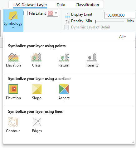
17. Check out the Symbology options. You can visualize the points by different attributes, including Elevation, Class and other attributes (vary depending on the data). You can also symbolize the layer as a surface rather than points. Try out the different symbology options.

Filtering LAS Points

The Filters group on the LAS Dataset Layer tab set allows you to change the display of the data and display selected classes or returns. Once the filter options have been chosen, any further analysis or symbology changes will honor the selected filters. This means any statistics run or files created will be created using only the filtered points.

18. Make sure the LAS Dataset is selected in the Content pane. Then in the LAS Dataset Layer tab, look for the Filters group. Click on the LAS Points drop down arrow to see the predefined LAS dataset filter options. Try some of the filters out and see how the points change.
19. Click on the LAS Points button to see all of the filter options. Try filtering by specific classes and/or returns and see the different results. The classification can vary greatly depending on the pre-processing of the data. Most Lidar point clouds include at least two classes: Ground and Unclassified (everything that isn't ground. The classification depends on the amount of processing that has been done.

Apply a Surface Constraint

Surface constraints are surface features stored in either geodatabase feature classes or shapefiles. We are going to use the shapefile of the boundary of the forest as Surface Constraint. This will clip the processing results to the forest boundary polygon. Note that the points won’t be visually clipped on the map in the LASD but should be clipped when displayed as a surface.

20. In the Catalog pane, right click on the LAS Dataset and select Properties. Click on the Surface Constraint tab.
21. Click Add and the plus button beside Surface Constraint to select the file. Find the boundary shapefile and select it. Keep height source as and select Hard Clip as surface type then click Add. Click OK to close the properties window.
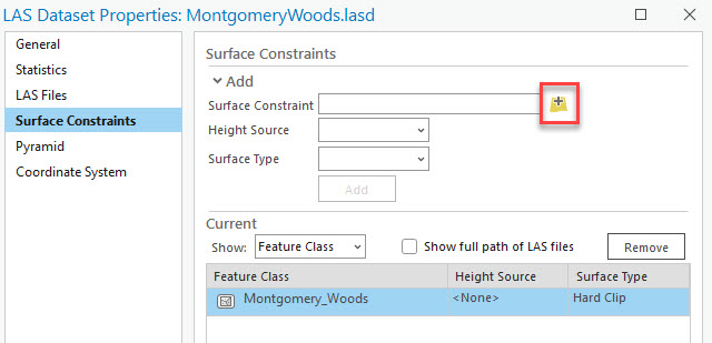
22. Select the Surface Constraints icon from the LAS Dataset Layer. Check the Surface Constraint to enable it.

Clipping LAS Data to a Feature - Extract LAS Tool

23. Make sure your filters are set to show all returns, as we want to clip or extract all of the lidar points. In your lab folder, create a new folder named Clipped_LAS.
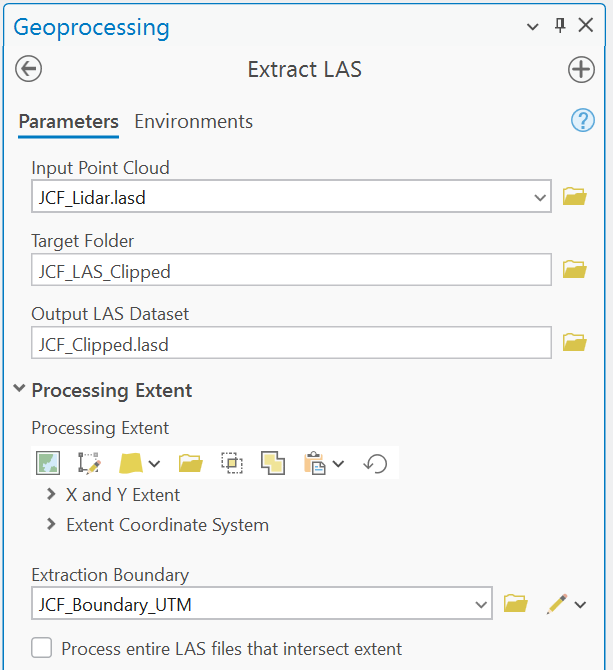
24. Navigate to the Extract LAS tool. This tool clips existing LAS files to a polygon boundary. The tool creates new LAS files as part of the clipping process.
25. Use the tool the extract the LAS points inside the boundary polygon. Use the Boundary polygon as the Extraction Boundary. Run the tool, it may take a while.
26. After the clipping has finished, review the properties and statistics for the LAS Dataset. Use ArcGIS Catalog view to accomplish this. Review and find the following information: How many different return categories are there? How many points total? Make note of the linear point spacing for all of the files and calculate the average point spacing the dataset. You will need this information for your lab turn in.

Evaluate Point Spacing - LAS Point Statistics As Raster

We are able to get a general idea of the point spacing and density by looking at the statistics. To further look at the point density distribution we will use the LAS Point Statistics As Raster geoprocessing tool. This tool allows you to see the spatial distribution of different lidar point metrics. It does this by characterizing the points that fall into each cell of an output raster. You can choose to summarize the points in several ways:

• Pulse count
• Point count
• Predominant return count
• Maximum returns
• Predominant class
• Intensity range
• Z-range (Elevation)

30. Before starting the process, check your LAS Dataset filters . In this case we will first evaluate the density (point or return count) for All Points, Launch the LAS Point Statistics as Raster tool by searching for the tool or
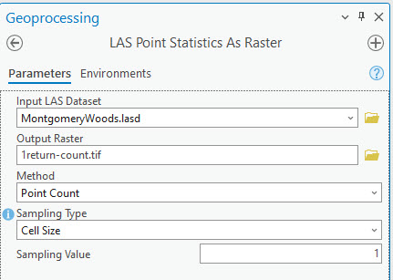
31. In tool window, select the JCF LASD as the Input LAS Dataset and save the Output Raster as return-count.tif. Select Point Count as the Method Set the sampling value to 1 (the units for this project are in meters) this will return the number of points within each 1 sq m pixel of the output raster. Run the tool.
32. A new raster will be created and appear on the map once the process has finished running. This raster display the point density per square meter. Adjust the symbology to better visualize the point density data (classified or color ramp). Look at the distribution of the points, for example are there any areas with significant gaps (no data)?

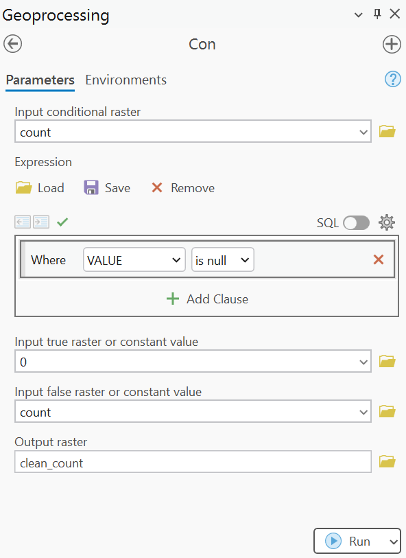
To properly calculate the percent canopy cover, we need to convert any resulting NoData cells to 0 so that subsequent operations treat a cell with no points as 0. We then need to clip the results to the forest boundary.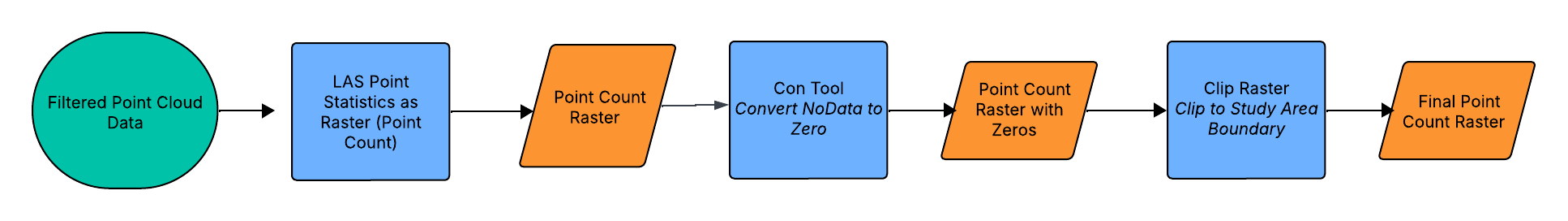

33. Use the Con tool to convert the No Data (Null Values) in the count raster to zeros.
34. Use the Clip Raster or Extract by Mask tool to clip and mask the previously created raster to the forest boundary polygon.
35. Under the properties for the final raster, look at the statistics for the point density data and copy/write-down the min/max/mean/SD stats for your worksheet.
36. Now filter the LASD data so only ground points are displayed. Rerun the LAS Point Statistics As Raster tool this time saving the file as ground-count.tif (keep all other settings the same). Repeat the above steps to determine the statistics for the point density data and copy/write-down the min/max/mean/SD stats for your worksheet.

Classify LAS by Height

The Classify LAS By Height tool reclassifies LAS points with class code values of 0 (never classified) or 1 (unassigned) based on their height from the ground surface created using LAS points with class code values of 2 (ground). Classifying points using height gradients from the ground surface can provide a useful way to visualize and filter the point cloud which can also aid the process of conducting more refined interactive classification. The tool defaults to classifying class codes 3, 4, and 5, which represent low, medium and high vegetation in the ASPRS specification for the LAS format, but the height settings may be changed based on project location and objective. We will use this tool to re-classify the

37. Run the Classify LAS by Height tool either through the Geoprocessing pane or from the Automated Classification tab under LAS Dataset in the main toolbar ribbon. Note this tool edits the original LAS file by changing the classification of specified points.
38. In the tool select the JCF LAS dataset as the Input and All Ground Points for Ground Source. Set the Height for the class codes as follows: Class 3 (Low Vegetation) : 2, Class 4 (Med Vegetation) : 5 and Class 5 (High Vegetation) : 100. Note that the Z units (elevation) for this data are in meters. This means all non-ground points between 0 and 2 m will be classified as “Low Vegetation”, between 2-5 m Medium and 5-100 m High vegetation. Set the Noise Classification to High Noise and check the Compute Statistics box, then run the tool. It may take a few minutes.
39. Once the process is complete the LAS dataset should update including the statistics. Review the statistics for the LAS dataset and change the symbology to classified to see the effects.
40. Finish filling out the worksheet and back-up your data for next week! To reduce the file size you can remove the LAZ and Original LAS folders. Be sure to back up the Clipped LAS folder!