Lab 6: Object Based Classification

Introduction

In this lab we will cover the ENVI object based classification workflow using the Feature Extraction tool. We will use the tool to classify a NAIP (National Agriculture Imagery Program) image

Learning Outcomes

• Perform Image Segmentation and collect training data for example based feature classification in ENVI
• Refine Classification Results

About the Data
The primary data in this lab is a NAIP image with four spectral bands (RGB NIR) and 0.6m spatial resolution. This image covers the north part of Arcata and was taken on May 31st, 2022.

Feature Extraction in ENVI

1. Download the data the most recent NAIP image of Arcata, CA that you can find (EarthExplorer is the easiest place to download NAIP imagery), download the image that covers the north western portion of Arcata. Move the data file into your original data folder and open ENVI.
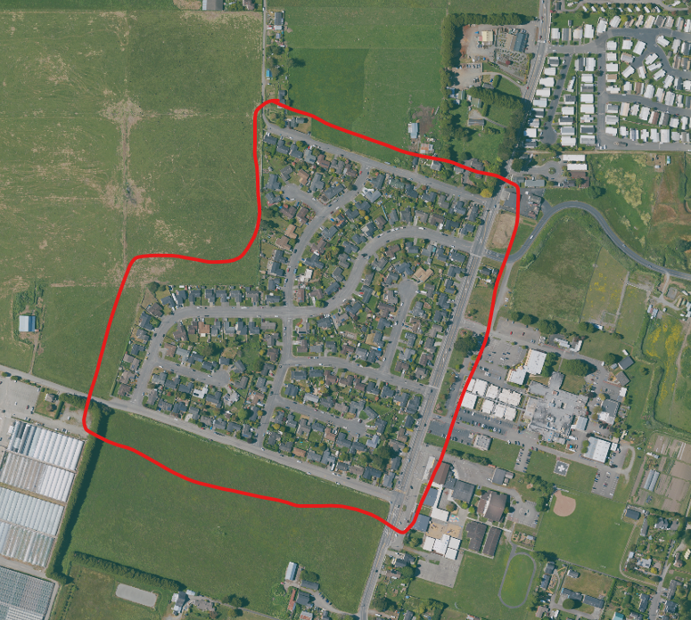
2. Open the file NAIP image (tif). Change the band combination to show a true color or NIR false color composite. To make the segmentation and classification process quicker we will create a Region of Interest (ROI) to limit the classification to small region. Create an ROI of an area of interest around the residential area to the west of Mad River Hospital ( 40.89728824°N,124.09524938°W). Use this ROI to build a raster mask (Build Raster Mask Tool) that can be applied in the classification workflow.
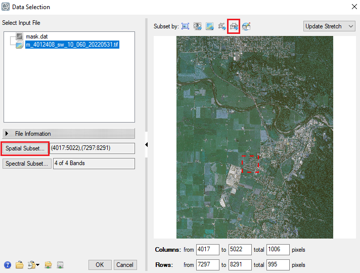
3. From the Toolbox, select Feature Extraction > Example Based Feature Extraction Workflow. The Data Selection panel appears. In the Input Raster browse and select the NAIP image. In the same window click the Spatial Subset button and use the ROI created in the previous step. Click OK. Selecting a Spatial Subset will limit the area the feature extraction will be applied to. Note that subsetting always results in a rectangular area, to limit the analysis to a specific polygon (with irregular geometry) we will need to apply a mask as well (next step).
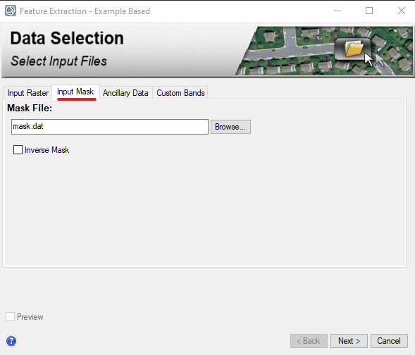
4. In addition to the spatial subset we will also apply the mask. In the Input Mask tab select the mask raster you created in the previous step. This will ensure only areas within the ROI polygon are classified.
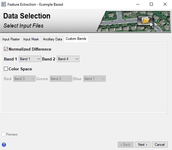
5. Before moving on in the workflow click the Custom Bands tab. This allows you to calculate custom bands that can be used in the segmentation and classification process. Click the Normalized Difference option and select the appropriate bands (Band 1 - Red and Band 4 - NIR for NAIP imagery). Click Next to start the segmentation process. ENVI will begin the process by stacking the data and computing statistics.
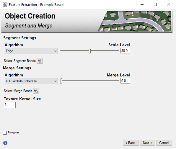
6. The Object Creation panel appears. This starts the segmentation process. Enable the Preview option. A Preview Window appears, showing the initial segments from the image, colored in green. You can change the RGB band combination of the input imagery to help you visualize.
7. Keep the segmentation method as Edge. Experiment with different bands for segmentation. By default all four of the original bands are used for segmentation, but using NIR or NDVI bands may be better for segmentation. Try different Scale and Merge values and see how they impact the segmentation. Try different values until you feel you have delineated the features adequately. Note that one of our goals is to delineate rooftops and compare pervious vs impervious.
8. When you are satisfied with the segmentation, click Next. ENVI creates and displays a segmentation image (called the Region Means image in the Layer Manager). Each segment is assigned the mean spectral values of all the pixels that belong to that segment.

Select Training Sample

When segmentation is complete, the Example-Based Classification panel appears with one undefined class (New Class 1). As you move the mouse around the segmentation image, the objects underlying the cursor are highlighted in cyan. You may need to click once on the image to activate this function.

9. Disable the Preview option, this will make the process smoother in the beginning.
10. In the Class Properties table, change the Class Name to Rooftop and press the Enter key.
11. Click on at least 20 different segments that represent rooftops. Try to pick a variety of sizes, shapes, colors, and intensities. The more training samples you select, the better the results from the classification.

The following are some tips for selecting training samples:
-Click again on a segment to remove it from selection.
-If individual segments are hard to discern from each other in certain areas, enable the Show Boundaries option to draw boundaries around each segment.
- If the segmentation image does not provide enough detail to determine if segments represent rooftops (versus a driveway or backyard, for example), uncheck the Region Means image in the Layer Manager. The original image will display instead.
- If you pan or zoom around the image, remember to click the Select icon in the main toolbar before selecting training regions.

12. Next, you should define several more classes that are not rooftop. In the Example-Based Classification panel, click the Add Class button . In the Class Properties table, change the new class name to Grass and press Enter. Select Grass in the left side of the panel, then select at least 20 training samples from the image that represent grassy areas such as backyards, fields etc.
13. Repeat the above steps for the additional classes, suggested classes include: Concrete (curbs and driveways) and Road (asphalt only), Trees etc.. Select at least 20 training samples each, and change the class colors as desired. Add any additional classes as you see fit. Once you have several classes turn on the Preview option to see how the classification will look based on the
14. Save an Example file button , and select an output folder and filename for the training regions you have defined. You can restore this file later if you want to continue where you left off.
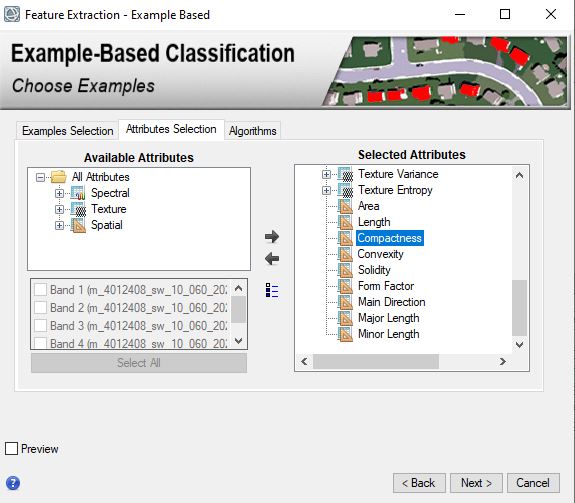
15. Select the Attributes Selection tab in the Example-Based Classification panel. For this tutorial, you can let ENVI determine the most appropriate attributes to classify with by clicking the Auto Select Attributes button . After a brief moment, the Selected Attributes column updates to show which attributes will be used. List of Attributes available and descriptions »
16. Use one of the Zoom tools in the toolbar to zoom to 100%. Enable the Preview option in the Example-Based Classification panel. A Preview Window appears with the current classification results. As you make changes to the training data, attributes, and classification settings, the classification results will automatically update. Move the Preview Window around the image or resize it to view results for different areas.
17. Disable the Region Means option in the Layer Manager, to hide the segmentation image. The original image will display underneath the Preview Window. Compare the preview classification to the original image.

Black segments are those that the classifier could not determine a suitable class for, so they remain unclassified. The Allow Unclassified option under the Algorithms tab controls whether or not to force all segments into one of the classes you defined.

18. If the classification needs improvement you can make adjustments in several ways: Adjust KNN Settings Select the Algorithms tab. Try increasing the Threshold value. The default value is 5 percent, which means segments that have less than 5 percent confidence in each class are set to "unclassified." As you increase the Threshold slider, the classifier will allow more unclassified segments. As you decrease the Threshold slider, the classifier forces more segments into classes, thus creating more opportunity for misclassification. Increase the Neighbors value to 3. A higher value takes into account more neighbors when choosing a target class and should reduce noisy or irrelevant features.
19. Collect More Training Samples If Necessary: If you have segments that are persistently being misclassified, you can assign them to known classes by following these steps: Select the Examples Selection tab. On the left side of the Example-Based Classification panel, select the class name that you want to assign the segment to. Ensure that the Select icon is active in the toolbar. In the image display, click on the segment to assign it to the selected class.
20. Define a New Class You will probably notice that some areas are incorrectly classified. Try creating a new class to capture any of these areas. In the Example-Based Classification panel, click the Add Class button . In the Class Properties table, change the class name, then select at least 20 training samples of the feature.
21. Continue to experiment with these options until you are satisfied with the classification of rooftops. Then click Next. In the next step, you will export the results to both a raster and vector file.
22. The Output panel lets you export various components of the supervised classification to raster images and/or shapefiles. By default, the classification image will include all of the classes that you defined. In the Export Vector tab, check the Export Classification Vectors option and be sure to include the attributes. Click the Export Raster tab. Enable the Export Classification Image option, and select an output directory to save the file. Click Finish. ENVI then adds a new classification data to the Layer Manager.
23. Create a pervious/impervious image. To do this review the classes and combine the classes into two broad categories of pervious and impervious (paved/rooftops) surfaces. You can either use the combine classes tool to permanently create a new dataset or simply change the colors of the associated classes.  Note that you will need to include a figure showing the original classification results as well as a figure showing the pervious/impervious results.
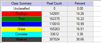
24. Right click on the classified image and calculate the statistics for the classified results. We will use this data to calculate the percent pervious vs impervious surface in the image. Copy the summary with pixel counts and classes into Excel.  Use this data to calculate the percent pervious vs impervious surface.
25. Now we will look at the vector file. Right-click the vector file generated from the classification in the Layer Manager and select View/Edit Attributes. This shows the attributes for all of the individual objects/features created in the classification process. Looking at this can help explore the type of attributes different features have. This could be used to later build a rule based classification workflow. Click on some of the different features and look at the attributes. Focus on some of the rooftops that appear to be correctly identified, see if they have common attribute values.
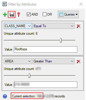
26. If a vector layer has an associated attribute table, you can filter the records by one or more attributes. Right-click the vector file generated from the classification in the Layer Manager and select Filter Records by Attributes. Create to filters, one so only the Class Name of Rooftop is selected. Then add a second filter to remove the small features that are clearly not rooftops, to do this use one of the area attributes and only select features that are larger than certain threshold. Experiment with different attributes to try and isolate only the rooftops in the image. When you are satisfied with your results note the number of records in the current selection (at the bottom of the window). This is an estimation of how many rooftops were detected in the neighborhood. Now we can export these selected features to a new shapefile. Click the Save icon and save the selected features in a new shapefile called "rooftops".
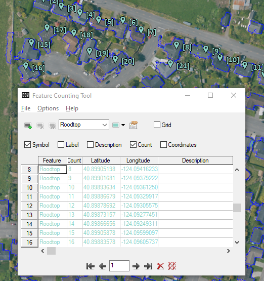
27. Use the Feature Counting Tool to manually count the Rooftops. Click the Feature Counting Tool button . A Feature Counting layer is added to the Layer Manager, and the Feature Counting Tool dialog appears with the following default settings. You can change the defaults, Feature 1 is the default name of the first feature group. The name appears as a label in the Image window view if the Label check box is enabled. To change the name, click in the name field and replace the name (with rooftops) and press the Enter key.
28. To count features, click on features in the view, or hover the cursor over a feature and press the Enter key. A record for the feature is added to the Feature Counting Tool table. Count all of the rooftops in the image using the tool. Note how many total rooftops you counted.
29. Prepare the maps/figures as stated below and review your results to make sure you have all of the necessary data to complete the lab.

Turn In