Lab 9 Part 2: Image Enhancements - Normalized Burn Ratio
Introduction
Normalized Burn Ratio (NBR)
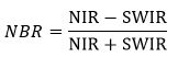
The Normalized Burn Ratio (NBR) was designed to highlight areas that have burned and to index the severity of a burn. The formula for the NBR is very similar to that of NDVI except that it uses the near-infrared band and the short-wave infrared band.
For a given area, NBR is usually calculated from an image just prior to the burn and a second NBR is calculated for an image immediately following the fire or one-year post fire. Burn extent and severity is judged by taking the difference between these two index layers. The meaning of the ∆NBR values can vary by scene and for the best results interpretation in specific instances should always be based on some field assessment. General ∆NBR classes have been developed, the higher the ∆NBR the higher the severity.
Learning Outcomes
Learn about various spectral indices and calculate spectral indices in ENVI.
Import vectors into ENVI and use vector files to subset data
Use Band Math Tool in ENVI to perform calculations with multiple bands or files.
Use the Raster Color Slice Tool to create a Burn Severity Map from a differenced Normalized Burn Ratio raster
Calculate the area of a class based on pixel count
Burn Severity Analysis (One-Year Post Fire)
For Part 2, we will be using Landsat 8/9 data to assess burn severity of the 2023 Smith River Complex Fires. The Smith River Complex was a series of wildfires in the Six Rivers National Forest that started on August 15, 2023. They fires were ignited by lightning strikes and eventually burned nearly 45,000 acres.
Create a folder on your Desktop named "Lab9_Part2" and
within the folder create three subfolders as below:
Originals
Working
Final
Locate the GSP 216 Google Drive lab data folder and navigate to the Lab 09 folder. Download the two "tarball" Landsat Level-1 files in the Part 2 folder. Extract the two Landsat files, make sure the Landsat files are extracted into separate folders.
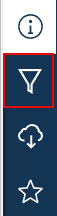
When the map first loads, there will be too many data records to load. Zoom in and you will start to see the various fire perimeter outlines. We will use the filter options to isolate the desired fire perimeters. Click on the funnel-shaped Filter Icon.
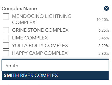
You can filter by various attributes, including fire name and year. You can find a full list and explanation of the available attributes under the View Full Details button. Since we are looking for a series of fires or complex, we will filter by Complex Name.
Under the Select Attributes heading, scroll down to Complex Name. Type Smith River in the search box for the Fire Complex Names and select the Smith River Complex from the dropdown list. Zoom in to the western California/Oregon border and you should see the outline of the selected series of fires.
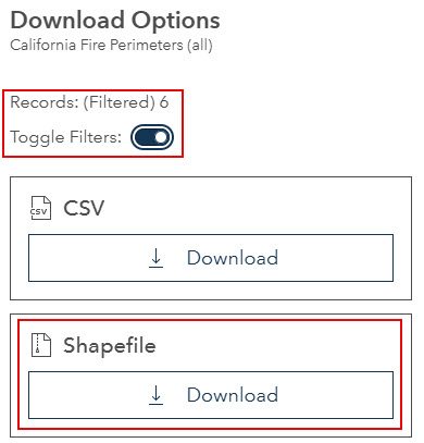
Click the Download Icon on the side of the map to select the download options and file type.
Under Download Options turn the Toggle Filters on, this will only download the filtered data selection. Click the Download Shapefile button. Once the file has been downloaded move and unzip the fire perimeter data into your Originals folder.
Open both the pre and post fire Landsat images (See Labs 6 and 7 for refresher on opening Landsat Level-1 data) by select File → Open and navigate to your Lab 9 Originals folder and open the metadata text file associate with each Landsat dataset ( ending in "_MTL.txt" ).
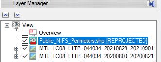
Open the Shapefile (.shp) of the fire perimeter from your Originals folder. In the layer manager the fire perimeter shapefile will say [REPROJECTED] behind the file name. This means the shapefile has a different coordinate system than the Landsat data and will need to be reprojected before we can proceed.
From the Toolbox, select Vector > Reproject Vector. In the Reproject Vector window, select the fire perimeter shapefile as the Input Vector.
Next we need to choose the appropriate Output Coordinate System for the file. This can be done by either browsing to select the coordinate system or by using the coordinate system from another dataset. We will use the other dataset method to have the shapefile coordinate system match the Landsat files. Click the From Dataset button . In the Data Selection Window select one of the Landsat files (it doesn't matter which one, they all should have the same coordinate system) and click OK. Now the coordinate system has been specified.
Select your Finals folder as the location to save the Output Vector and save the file as "fire_perimeter.shp". Click OK to run the reproject tool. When it is complete the new re-projected shapefile will appear in the layer manager and should no longer say [REPROJECTED].
Open the Data Manager . Remove the original shapefile by click on the file name in the data manager and clicking the Close File icon. Close the Data Manager when you are done.
Radiometrically Calibrate and Subset Images by Importing Shapefile
Now we will explore the Normalized Burn Ratio (NBR). We will use the NBR to look at the burn severity of a recent fire. We will be looking at two Landsat 9 scenes of the area, a pre-fire scene and a one-year post-fire scene. The images are Level 1 data that were acquired from EarthExplorer.
If you load the fire perimeter shapefile and discover you have more polygons than just your desired fire perimeter watch the video below
Optional Video: How to extract selected polygons
Change the band combinations of both of the images to make the burn area more visible. Select the Shortwave Infrared preset false color band combination (Red - SWIR 2, Green - NIR, Blue - Red). The burn areas should now be more clearly defined on the post-fire image. Make note of file name/date of the pre and post fire images, you will need this information for the next steps.
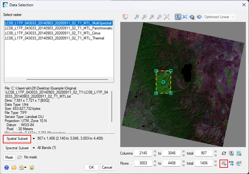
Now we are going to perform radiometric calibration and convert the data to Top of the Atmosphere (TOA) reflectance. In the Toolbox, open the Radiometric Calibration tool. In the window click to select the Input Raster. In the Data selection window select the multispectral pre-fire image (look for the earlier date in the file name). Before moving to the next window click the Spatial Subset button. You should now see a preview of the image. Click the Subset by Vector icon and select the fire perimeter shapefile. ENVI will show a preview of the subset, click OK to move to the next step.
The above screenshot is an example from the 2014 King Fire, the data for this lab will be different.
In the Radiometric Calibration window select "Top of the Atmosphere Reflectance" as the calibration type. Name your output file file "prefire.dat" and save it in your Lab 9 Final folder. Leave the Scale Factor and Output Data Type as the defaults.
Repeat the above steps to radiometrically calibrate the post fire image, be sure to select the multispectral image with the later date, and to subset with the same shapefile and use the same calibration settings. Save this image as postfire.dat in your Final folder. You should now see two radiometrically calibrated, subsetted images in your viewer (pre and post fire). Turn the layers on and off to see the differences between the images.
Example calibrated pre and post fire images from the 2014 King Fire.
Before you go on to the next steps verify that both your images are subset to the exact same geographic area and that both subset images have been calibrated to Top of the Atmosphere Reflectivity. You can do this by turning on and off the subset layers and confirming that they have both been cropped to the same extent. You can check the image description in the metadata to confirm that it has been calibrated to Top of the Atmosphere Reflectivity.
Remove the files that are no longer need, open the Data Manager by clicking the icon or selecting File → Data Manager. Remove all files from the data manager except for the subsetted images and shapefile ("PostFire.dat, PreFire.dat" and the fire perimeter shapefile), to do this select all of the files you would like to remove the "Close File" icon . This will make it easier to manage our data in the next steps. Close the Data Manager.
Create Normalized Burn Ratio (NBR) Rasters
From the Toolbox, select Band Algebra → Spectral Indices or type "Spectral Indices" in the Toolbox and open the Spectral Index tool. The Spectral Indices dialog appears. Select the PreFire.dat is your Input Data and click OK.
Now we will select the desired Spectral Index from the Spectral Index list: Normalized Burn Ratio. Name your output raster "PreFireNBR.dat" and make sure it is saved in your Lab 9 "Working" folder. Check the Preview box and you should see a new view open up with a preview of the NBR results. Click OK and by default the NBR image will appear in the viewer.
Repeat the above steps to create a post-fire NBR using the subsetted post-fire image. Name your output NBR raster "PostFireNBR.dat" and save to the "Working" folder. The post fire NBR image will appear in the viewer. The
dark burn scar should be visible in the post fire NBR.
Creating a Differenced Normalized Burn Ratio (ΔNBR or DNBR) Raster
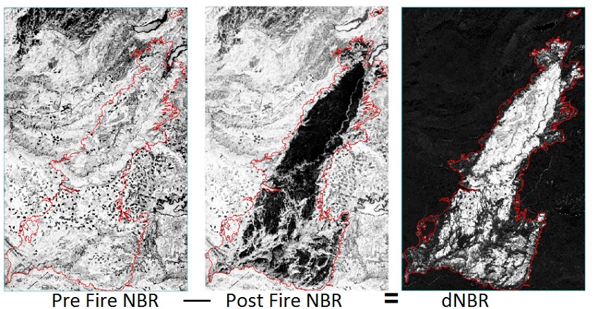
A differenced normalized burn ratio (ΔNBR or dNBR) is a burn-severity raster that measures absolute change in the NBR between two time periods. In the
ΔNBR raster, higher pixel values (brighter areas) indicate a higher burn severity. The dNBR is created by subtracting the Post Fire NBR from the Pre Fire NBR.
A dNBR value close to zero indicates little change or unburned landscape.
From left to right: Pre fire NBR, Post Fire NBR, dNBR from the 2014 King Fire.
From the Toolbox, select Band Algebra → Band Math or type "Band Math" in the Toolbox and open the Band Math tool. The Band Math window will open.
Enter the following expression: float(b1 - b2) and click OK. The Variable to Bands Pairings window will open, this is where you will we tell ENVI which bands or data to use for the variables (b1 & b2).
For Band 1 (B1) select the "PreFireNBR.dat - Normalized Burn Ratio" by clicking on this file in the Available Bands List. For Band 2 (B2) select the "PostFireNBR.dat - Normalized Burn Ratio".
Click Choose by Enter Output Filename and name your file "dNBR.dat" and save it in your "Final" folder. Click OK to run the process.
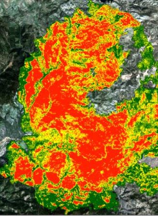
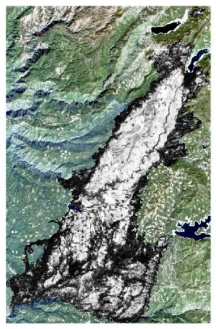
The differenced normalized burn ratio raster is now in your viewer. Areas that are dark indicate areas with minimal change (low severity or unburned), larger values appear lighter and indicate significant change (high severity) between the images.
To limit the analysis to inside the fire boundary, we will mask the dNBR using the fire perimeter shapefile. In ENVI this can be achieved through masking. In ArcGIS you can use the clip functions to achieve
similar results. After masking, the Raster Color Slice Tool in ENVI will be used to create the burn severity classes, this can also be done with the Reclass tool in ArcGIS.
For this exercise we will be using ENVI to create the classification.
To mask the dNBR file, select File → Save As → ENVI/TIF. In the Data selection window select the file you want to save (dNBR.dat file) and then click Mask. Select the Fire Perimeter shapefile as the Mask. Click OK twice.
Keep the file type as ENVI. Now we need to set the data ignore value. This is the value that will be used for the mask areas (outside of the fire perimeter).
ENVI ignores these values, which means they are not displayed or included in calculations or analyses. Use -9999 as the Data Ignore Value. Save the file as dNBR_masked.dat.
Example masked dNBR from the 2014 King Fire
The new masked dNBR file should now be in your window (see example above), with only the area within the fire perimeter visible. Turn off or remove the other NBR and dNBR layers to ensure the file has been properly masked.
Create Severity Layer
Now we will create burn severity classes using the Raster Color Slice tool. Right click on the masked dNBR file and select New Raster Color Slice.
In the data selection window select the masked dNBR file and click OK. In the Raster Color Slice window select New Default Color Slices .
Now we are going to classify our dNBR values into five discrete burn severity classes or slices. Change the number of slices to five and change the colors here if you like, click OK.
Change the min and max values for the "slices" (classes) to the values in the table below. Keep the first slice minimum value as the default (the minimum value for the image) and the maximum value of last slice as the maximum value recorded.
For example, leave the minimum value for the first class as the default and set the maximum value to 0.1, then continue to the next class.
These values for the burn severity classes are derived from : Key, C. and N. Benson. "Landscape Assessment: Remote sensing of severity, the Normalized Burn Ratio; and ground measure of severity, the Composite Burn Index." In FIREMON: Fire Effects Monitoring and Inventory System, RMRS-GTR, Ogden, UT: USDA Forest Service, Rocky Mountain Research Station (2005).
ΔNBR Range
Burn Severity Class
<0.1
1 - Unburned
0.1 to 0.27
2 - Low-severity
0.27 to 0.44
3 - Moderate-low severity
0.44 to 0.66
4 - Moderate-high severity
> 0.66
5 - High-severity
The above histogram is an example from the 2014 King Fire data. The shape of the histogram and histogram minimum and maximum values will be different for your data.
Click on the Save icon, selecting Export as Class Image. This will save the classified dNBR as raster file. Save the file as severity.dat in your Final folder. This will be the file you use to create the burn severity map.
Then click the Save icon again and this time select Save Color Slice to File. Save the file as "burnseverity" in your Finals folder. The file type is .dsr and this file just saves the colors and value ranges for the slices/classes, not the actual image file. This
allows you to import the file and use the same values ranges and colors with other data sets. Click OK and then close the Raster Color Slice Window.
Calculating Area of Burn Severity Classes
Right click on the Classes or Slices folder icon under the burn severity layer and select Statistics for all Classes/Slices. In the next window select the severity.dat file as the Associated Data Input File and click OK.
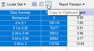
The Classification Statistic window will open. The Class Summary table will display the pixel count for each of the burn severity classes. Highlight the classes and pixel counts and copy this data into a document or spreadsheet.
Now that we know the number of pixels in each class, we can calculate the area. The only additional information we need is the spatial resolution of the raster. To confirm the spatial resolution, right click on the file name (severity) in the Layer Manager and View Metadata and confirm the → Pixel Size (X,Y) and units. This will be used to determine the area of a single pixel.
Example: Calculating Area of Classes
Area in Acres = ([Pixel Count] * Spatial Resolution 2)/4046.86 m2/ac
First determine the spatial resolution of the raster and the number of pixel in the class or category
Area of One Pixel: 30m x 30m = 900 m2
Count of Pixels: 10,500
Total Area = 900 m2 x 10,500 = 9,450,000 m2 - Note that 1 acre = 4046.86 m2
Using the above method, calculate the area in Acres of each of the burn severity classes, note that Excel is an easy way to do this.
We have all of the information and data needed to complete our burn seveirty map. Verify that all of your files are saved in your Finals folder and close ENVI.
Creating Burn Severity Map in ArcGIS Pro
Now we will open the files in ArcGIS Pro to create a Burn Severity map. In many cases you may want to determine the area of a class/category in an image. This can be done easily if you know the spatial resolution (pixel size) and the number of pixels in the class. We will map our burn severity and calculate the area in acres of each of the burn severity classes.
Open ArcGIS Pro and create a new map project and save it in your finals folder. In the Catalog Pane connect to your Lab 9 folder. Remove the default base maps.
Before adding the data we will build an attribute table for our severity raster before moving forward. In the Geoprocessing Pane (can be located by going to Analysis → Tools), search for the Build Raster Attribute Table tool. Start the tool and select the severity.dat file from your Final folder and click Run. This process creates an attribute table for raster files that include the class value and
the number of pixels in each class. By default many classified raster files created in ENVI do not have attribute tables that ArcGIS can read. The Build Raster Attribute Table tool takes care of this issue.
Now add the Severity.dat (if it hasn't been automatically added), PostFire.dat Landsat image (or pre fire Landsat image if you prefer) to your map project. The severity file should be on-top of the true color Landsat image.
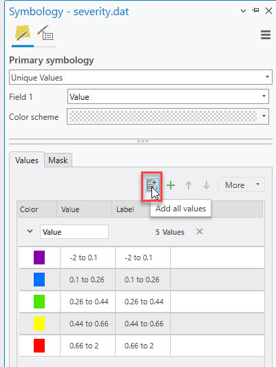
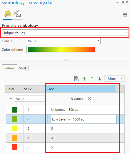
Select the "severity" layer and go to the symbology for the layer. Change the symbology type from "Color Map" to "Unique Values". Change the color scheme, typically color schemes from green, yellow, orange to red are used, where red indicates high-severity burn areas and green unburned. You may choose a different color scheme, just be sure there is enough contrast between the colors.
Next click the Add All Values Icon below to add all of the classes or values in the attribute table to the map. You should now see the burn severity classes on your map.
Now update the Label column for each item so that the label for each class is the burn severity class name followed by the area in acres (refer to your calculations in previous steps for the class names and acerage). Leave the Value column as is.
Now we will make the final burn severity map layout . Add a New Layout (Insert → New Layout). Add a Map Frame to the newly created layout (Insert → Map Frame). It doesn't matter what size or where you place your map frame at this step. we will adjust the size and zoom level in the next.
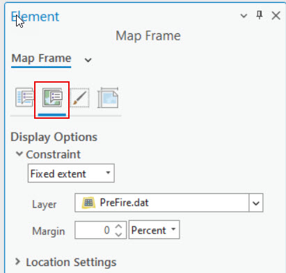
Right click on the map frame and select properties. The Map Frame Element tab pane opens on the side. In the Display Options tab, under Constraint select Fixed Extent and select the Landsat image. This sets the view of the map frame to show exactly the area of the Landsat image and the burn severity layer. Now adjust the map frame until it fills the majority of the paper.
Now we will make the final visual adjustments to the images. Make sure you Landsat image is displayed as a true color image in the background with the burn severity layer on top. Use the displays tools under Raster Layer tab to fine tune the contrast and brightness of your Landsat image if desired.
Center your map frame from side-to-side (horizontally) by going to the Map Frame tab and selecting Align. Then turn on Align to Page option and select Align Center.
Add a legend for the Burn Severity class layer. Select the severity file in the Contents pane and select Legend and add a legend to the mapTo change the legend style right click click on the legend and select “Properties”. I suggest replacing the word "Legend" with "Burn Severity" or something similar or removing the text all together. The legend should include only the burn severity classes and the corresponding area in acres. Read more about the Arrangement and formatting of the legend items
Now add a scale bar, title, north arrow, legend, data source and map author to your map layout. All of these can be found under the Insert tab when in Layout view.
Example burn severity map from the 2014 King Fire
When you are happy with your map export it to a PDF or image file (PNG or JPG). In the main toolbar ribbon select Share and then click “Export Layout ”. Select PDF or PNG/JPG as the type and make sure the resolution is set at 300dpi and save it in your “Final” Lab 9 folder. Save your map project file in the same folder.
Burn Severity Map PDF (Upload to Canvas)
Burn Severity Map should include:
True color Landsat Base Image
Classified Burn Severity layer clipped/masked to fire boundary
Scale, Title, North Arrow and Legend with class names and acreage and the Fire Perimeter (optional), data sources and map author.
Contact Info
Humboldt State University
1 Harpst Street Arcata, CA 95521
skh28@humboldt.edu


 The above screenshot is an example from the 2014 King Fire, the data for this lab will be different.
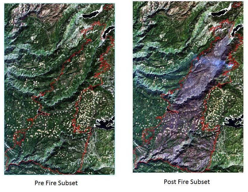 Example calibrated pre and post fire images from the 2014 King Fire.
  . This will make it easier to manage our data in the next steps. Close the Data Manager.
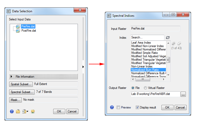
 From left to right: Pre fire NBR, Post Fire NBR, dNBR from the 2014 King Fire.
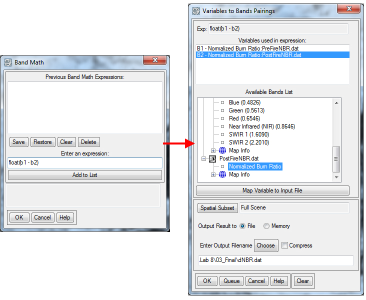
 Example masked dNBR from the 2014 King Fire
 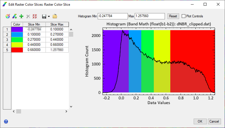 The above histogram is an example from the 2014 King Fire data. The shape of the histogram and histogram minimum and maximum values will be different for your data.
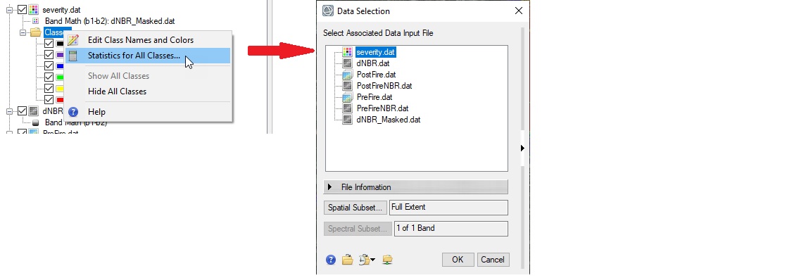
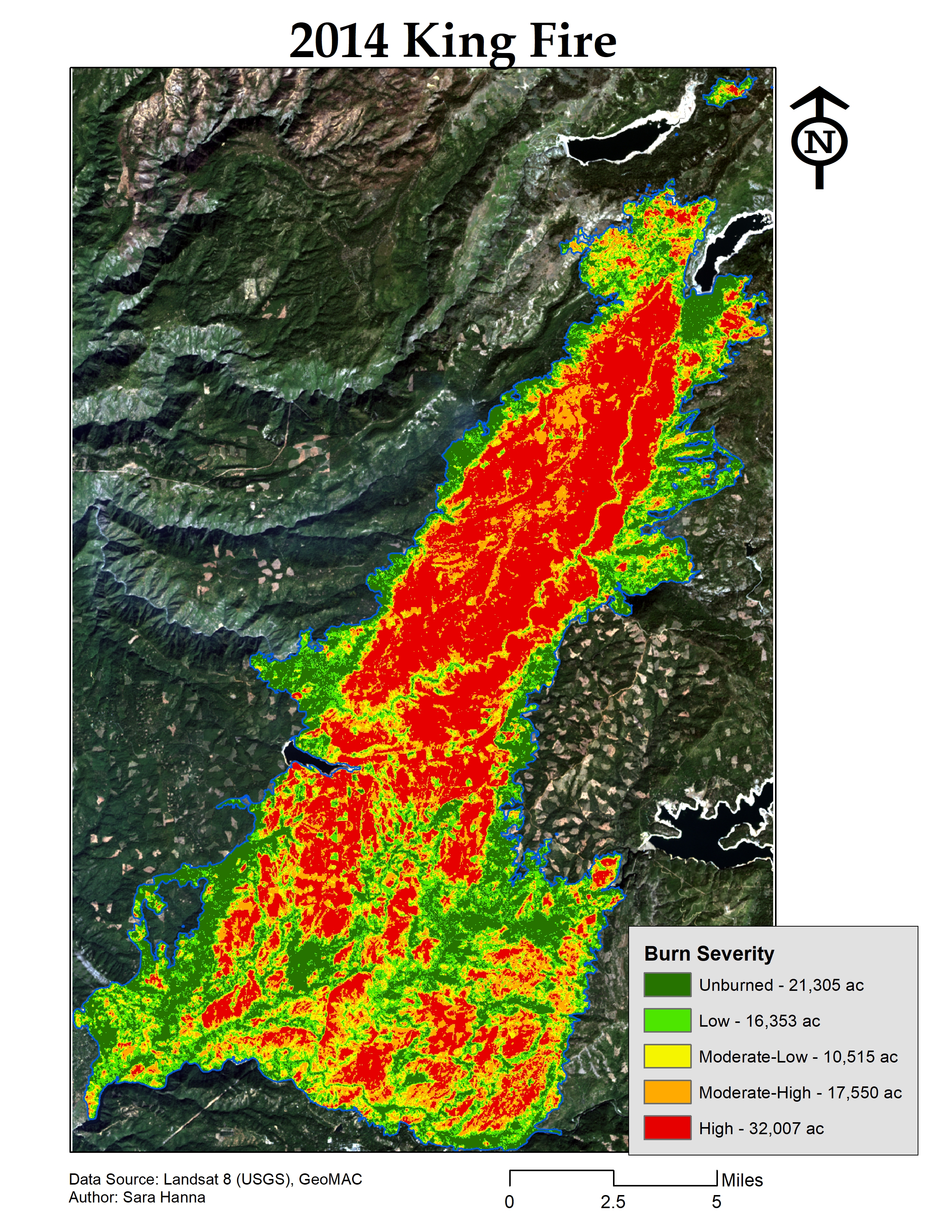 Example burn severity map from the 2014 King Fire