In this lab we will explore digital imagery with different spatial, spectral, radiometric and temporal resolutions.
It is important to understand the characteristics of remote sensed data so you can select, and process digital images appropriately.
In this lab we will be working with four types of imagery: MODIS, Landsat, PlanetScope and NAIP.
About the Data
The majority of the data was acquired in the end of August 2022 in California (the NAIP image was taken two years prior in 2020). The images focus on the early days of the Six River Complex Fire located near the town of Willow Creek, CA. The series of fires started on August 5th, 2022 after a lightening storm ignited multiple fires across the area. The fires continued to burned for several weeks but were largely controlled quickly..
Note that the NAIP and MODIS data were re-projected from their native projections and the MODIS data has a different project than the others.
Determine the spatial, spectral, radiometric and temporal resolution of datasets
Understand the concept of resolution and how it relates to digital images and file size
Become familiar with ENVI functions, including viewing metadata, portal views and functions.
Create, analyze and export Regions of Interest (ROIs) in ENVI
Manage geospatial data
Create and export a simple map in ArcGIS Pro with raster and vector data.
Setting up your Workspace
First we need to set up our workspace, transfer the data and open the data in ENVI.
Create a Lab 5 folder on the desktop and create the following sub-folders:
Originals
Finals
Open up your favorite web browser, log into myHumboldt and navigate to your Humboldt Google Drive. Locate the Lab Data folder withing the GSP 216 Remote Sensing folder. In the folder navigate to the Lab 5 Data folder, locate the file “Lab5_data.zip”. Right click on the file and select “Download”.
Open the Downloads folder and right click on the file “Lab5_data.zip” and select “Extract All”. When prompted to "Select a Destination and Extract File", select Browse and select your Lab 5 Originals folder. Click Extract. Now the files have been uncompressed into you Originals folder and are ready to open. This folder contains the data and associated metadata files for the four images.
Start ENVI 5.6 and open the raster file “Landsat.dat” which should be located in your Originals folder. You should now see the true color Landsat image in your main viewer.
View Metadata in ENVI and as Text Document
The Metadata Viewer in ENVI provides a variety of information about the data file. Typically this information is stored in the ENVI header file (.hdr). This can include general information about the file (location size, etc.), the coordinate system and the spatial and spectral resolution. This is a good place to start when investigating the properties and resolution of a dataset.
Open the Metadata Viewer by right clicking on the file name in the Layer Manager and selecting "View Metadata". The Metadata Viewer will now open.
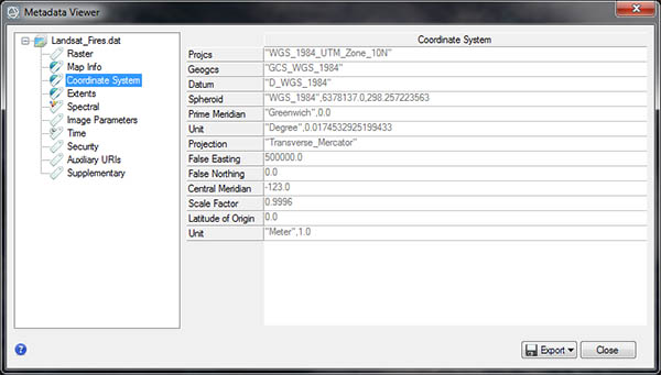
Use the metadata viewer to determine the spatial and spectral resolution of the image, you will need this information for your lab report. The spatial resolution can be found in the "Map Info" section
under "Pixel Size X and Y" and associated "Units". Spatial resolution should be reported as the length of one side of the pixel in meters.
Spectral resolution can be found under the "Spectral" tab. Depending on the sensor and metadata there may be varying amounts of information in the Spectral tab. At a minimum, you should be able to determine the number of bands present in an image. Spectral resolution should be reported as the number of bands and the range of the electromagnetic spectrum they cover (either by name or wavelength). Use the internet to research the spectral bands if all of the information is not present in the metadata.
Click through all of the tabs on the right and review the available metadata. You may want to make note of the coordinate system and the file size.
Outside of ENVI, navigate to your Lab 5 Originals folder and open the Landsat metadata text file ("Landsat_metadata.txt"). By default it will open in Notepad. This is the metadata file that is provided with the Landsat data when you download it from a source like EarthExplorer. Review the metadata and find the acquisition date of the image. An easy way to do this is to use the "Find" function (Ctrl + f) and type in date. There may be more than one date, if there are multiple dates look for the words "acquisition date" or "date acquired". For MODIS data this is usually listed as "Range Date Time".
Research the radiometric resolution and temporal resolution (also known as return time) of the sensor by visiting the sensor website or by using an internet search engine to locate the information. Typically radiometric resolution is reported in bits (8-bit, 12-bit, 16-bit). Radiometric resolution is also sometimes referred to as "Data Quantization". Regardless of the terminology used, it should be reported in bits. Temporal resolution should be reported in days/weeks/years etc.
Zoom in until you can see each pixel. Now zoom out until you can make out an identifiable feature. Note what details you can make out in the image, i.e. individual trees/plants, roads, lakes or other features. You may want to change the brightness of the image to make it easier to interpret. Zoom to the full extent of the image. This will give you an idea of the footprint or geographic area cover by each image.
View and Research MODIS, PlanetScope and NAIP Data
In the same viewer open "PlanetScope.dat". Repeat steps 5-11 for the PlanetScope image.
In the same viewer open "NAIP.dat". Repeat steps 5-11 for the NAIP image.
In the same viewer open "MODIS.dat" Repeat steps 5-11 for the MODIS image, but note that you will need to research the all of the resolutions for MODIS online. Note that we are viewing a subset of the MODIS data, one for the bands with 500m spatial resolution. You may summarize the resolutions for your table.
View Portals and Tools
When you have multiple files or layers open in ENVI, you can explore and compare them using a portal. The portal tool opens a subset of the Image window view that you can move and resize within the view. You can create multiple Standard Portals per view. There are also Blend, Flicker and Swipe view tools that allow you to compare two data layers. These tools by default will always compare the top two files.
Rearrange the layers, in the Layer Manager, drag to NAIP image to the bottom. Now the MODIS image should be on top, followed by the Landsat, PlanetScope and NAIP on the bottom.
Use the Blend Flicker and Swipe tools to compare the four layers. Click the "Portal" icon in the toolbar to open a portal view. The portal viewer will open and you will see the Landsat image in the Portal window and the MODIS image behind. The Portal tool uses the first non-portal layer in the Layer Manager as the display layer, and the second layer as the source in the Portal window. Use the cursor to drag the portal view around, you can change the size of the portal window by dragging the corners to re-size. You can open up multiple portal views at a time to display different layers.
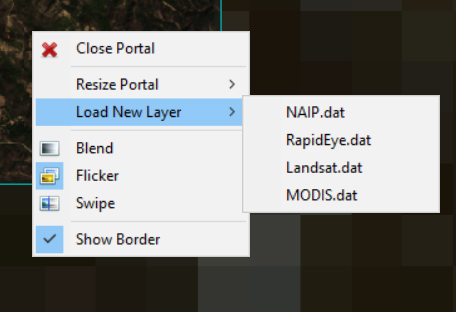
Right click on the "PlanetScope" file in the Layer manager and select "Zoom to Layer Extent". Then right click again and select "Display in Portal". A new portal window will open showing the PlanetScope layer in the window. Right clicking on the Portal window gives you the option to Close the portal, Resize or Load a New Layer in the current Portal window.
When you are done exploring close the portal windows by clicking on the "X" in the top right hand corner or right click on the portal view in the Layer Manager and select "Remove". .
Now let's check out Blend, Flicker and Swipe tools. The "Blend"tool creates an animation that blends or fades between the two selected layers, the "Flicker" tool creates an animation that switches between the two layer and finally the "Swipe" creates an animation that swipes between the two layer.
Turn off the the comparison tools by clicking on the icon again or right clicking on the "View Flicker/Blend/Swipe" in the Layer Manager and selecting "Remove".
Let's compare the four images side-by-side. To do this select Views → 2x2 Views. This creates four views equally sized views. Re-arrange the files so each of the images is in a separate view. This can be accomplished by dragging and dropping the files from the layer manager into the view window. Use the "Link Views" tool to geographically link the images (Views → Link Views → Link All). Not all of the images cover the same area (they have different footprints). Zoom in on the NAIP image or right click on and select "Zoom to Extent". Compare the different spatial resolutions of the four images in the side-by-side views.
False Color Composites
Focus your viewer on the actively burning fires by Willow Creek, CA. Currently the area is obscured by smoke. In your viewer with the Landsat image, click the Data Manager iconin the main toolbar. The Data Manager displays all files that have been opened this session and allows you to reopen the files from this menu. Find the file “Landsat.dat”, now we will select the band color combination. Click the box on next to “SWIR 1”, it should turn red after it has been selected. Next click the box next to “Near Infrared (NIR)” and it should turn green and lastly click the box next to “Red” which will turn blue. This is an infrared false color composite displaying the SWIR1, NIR and Red wavelengths. You will notice that some of the smoke has disappeared and the boundaries of the fires are more visible.
Use the Blend, Flicker and Swipe tools to animate between the two Landsat layers (true color and false color) to see the differences.
Now let’s change our view to display a different infrared false color composite. In this false color composite we will only be visualizing the shortwave and near-infrared portions of the spectrum and none of the visible spectrum. Right click on the top "Landsat.dat" file in the Layer Manager and select "Change RGB Bands".
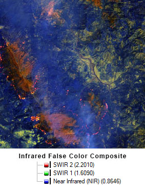
In the "Change Bands" dialog, click the box on next to “SWIR 2” first, it should turn red. Next click the box next to "SWIR 1” and it should turn green and lastly click the box next to “Near Infrared (NIR)” which will turn blue. Click "OK" and now you should see a new false color composite in your view (see example image to the right). In this composite, healthy vegetation looks blue, dry/bare ground appear shades of yellow-green and recently burned areas appear red. The fire boundaries should now be clearly visible as well as "hot-spot" or actively burning areas of the fire.
We will look at one more false color composite. Right click on the top "Landsat.dat" file in the Layer Manager and select "Change RGB Bands". Click the box on next to “SWIR 2” (red), the click click the box next to "SWIR 1” twice, it should turn green and blue. Now we will only be visualizing the two SWIR wavelengths. Click "OK" and now you should see a new false color composite in your view, where the majority of the image appears grey toned
and the burned areas appear red.
Use the Blend, Flicker and Swipe tools to animate the layers to see the differences. You can also make false color composites that include the Thermal Infrared bands as well.
Right click on the NAIP, MODIS and PlanetScope images in the layer manager and select change RGB bands. Explore the spectral bands available and experiment with different false color composites for each of the four images. When you are done, remove all of the files except the false color Landsat image and close all of the views except the one with the Landsat image. Learn more about MODIS band combinations
Create Regions of Interest (ROI)
Regions of Interest (ROIs) allow you to select specific areas of rasters. The ROIs can be saved and used for a variety of purposes, including calculating statistics, area and subsetting images. ROIs can
be created from geometry or by pixels. ROIs are vector files, which are coordinate-based data models that represent geographic features as points, lines, and polygons. Each point feature is represented as a single coordinate pair, while line and polygon features are represented as ordered lists of vertices. While ROIs are an ENVI Vector data type, they can also be easily be exported as Shapefiles to work with in other geospatial applications.
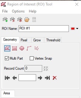
We will start first by creating a practice Region of Interest. To create a new Region of Interest (ROI) click the Region of Interest (ROI) icon on the toolbar or right click on the Landsat file and select new Region of Interest. The ROI Tool window will now appear. Watch the video at start of this section for a more detailed overview of the process.
Use the Go To tool to navigate to 40.56538369°N,123.16548292°W, then zoom into between 200-400%. You should now see a small lake near Hayfork, CA. We will use the ROI tool to digitize the small Ewing reservoir.
Click the Polygon icon . Click to mark the vertices of the polygon or polyline, or click and drag to draw the shape of the lake. To complete the shape, right-click and select "Complete and Accept Polygon ". Until you "accept" the shape, it appears translucent and you can edit its size or vertices, or move it. Once accepted, a shape appears in solid color.
Now delete this practice ROI by clicking on the Remove ROI icon . This will delete the selected ROI.
Now click new ROI icon to create a new ROI. Navigate to either Lake Shasta or Trinity Lake and rename the ROI the appropriate lake name. This time instead of manually digitizing the lakes we will use the Magic Wand Tool. The Magic Wand tool uses "seed" pixels to then select similar color features surrounding it. Using false color composites can improve the results by selecting composites with high contrast between the features. The tools uses the RGB values displayed on the screen to make the selection. This tool facilitates drawing ROI polygons around complex objects such as clouds, tree crowns, and lakes.
With the Region of Interest (ROI) Tool displayed, hold down the Ctrl key and click on a pixel inside one of the lakes. An initial polygon is drawn, and the Magic Wand Parameters dialog appears. You can adjust the threshold and experiment with other parameters to better refine the shape of the object. Once you are happy with your ROI selection (aim to select the entire lake but no other features), right click and select "Accept Multipart". The outline should turn a sold color.
A nice feature of ENVI is that it automatically calculates the area of ROIs. In the ROI Tool Window click on the "Area" tab. By default the area is shown in pixel. Click on "Units" in the Area toolbar
and change the units to Acres. You should now see the area of the ROIs listed in acres, write this information down or click the "Save" icon to save the area of the ROI as a text file or copy and past the area into a document.
Now we will create new ROIs that represents the boundaries of actively burning Six Rivers Fire and area burned by the fire. Navigate to the Willow Creek area. Note that on the fires continued to grow significantly after the images was taken. Click the new ROI icon to create a new ROI. Name the new ROI "SixRiversFire". Make sure you are using one of the infrared false color composites to more easily see the fire perimeter.
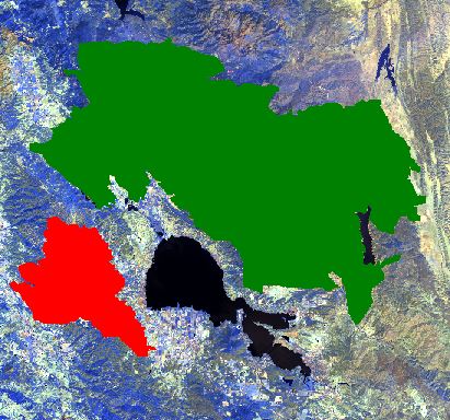
We will now use the polygon tool to start manually digitizing the approximate boundaries of the several fires that made up the Six Rivers Complex on this date. Click the Polygon icon and check the Multi Part box. This will allow you to create several separate polygons in one ROI. Click to mark the vertices of the polygon or polyline, or click and drag to draw the shape. To complete the shape, right-click and select "Complete and Accept Polygon Part". Until you "accept" the shape, it appears translucent and you can edit its size or vertices, or move it. Continue digitizing additional polygons until you have digitized the current fire boundary. There should be multiple separate polygons for the fires. When you are satisfied with the ROIs, press right click again and select "Accept Multi Part". Once accepted, a shape appears in solid color. Your fire boundaries do not have to be perfect, but they should be a good approximation of the fire location and spread at the time the image was taken.
Click on "Units" in the Area toolbar
and change the units to Acres. You should now see the area of the ROIs listed in acres, write this information down or click the "Save" icon
to save the area of the ROI as a text file or copy and past the area into a document.
Example of fire perimeter ROIs for a different fire
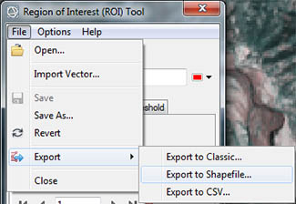
You can save and export your ROIs for future use. We will export our ROIs as a Shapefile (.shp) so we can use and view the file in ArcGIS or other applications. We will export the fire and lake ROIs separately. In the ROI Tool Window select File → Export → Export to Shapefile. Select the Six Rivers Fire ROI only and name the file "boundaries" and save it in your Lab 5 "Finals" folder. Click "OK" and ENVI will export the file to a Shapefile format.
Repeat step 39, but this time select only the Lake ROI and save the shapefile with an appropriate name in your finals folder. Wait for all of the files to export, it may take a few minutes to fully complete. You can close ENVI once the file has been exported (you can check your finals folder to be sure the files have been exported.
Manage Data and Create Map in ArcGIS Pro
Create a map that either shows the Six Rivers Fire Perimeters or one that shows the lake levels in either Shasta or Trinity Lake.
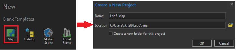
Start ArcGIS Pro. When working on campus you may begin working immediately if you are working from your personal computer you may need to sign in with your ArcGIS Online account (If you don’t want to sign in each time, check “Sign me in automatically”). Select a new Map Template and create a new project named Lab5-Map in your finals folder for the lab, uncheck the box so a new folder isn't created.
Let’s make sure ArcPro knows where your files are located. In the Catalog Pane, expand Folders and see if your data folder is shown. If not, don’t worry – your files are still where you left them! Right click on Folders
and select Add Folder Connection.(Don’t see the Project Pane? Click View | Catalog |
Catalog Pane.). Add your GSP 216 folder or Lab 5 as a folder connection. Once you’re connected to your folder, you’re ready to add data to your map.
Before we add any data, let's move the Landsat image from the Originals folder to your Finals folder. Click on the Catalog pane on the side and expand the folders. Find the Landsat.dat file in your Originals folder and drag it into your Finals folder.
This means all of the data necessary for your project will be in your finals folder which will make it easier to back-up.
Click the add data button to add a data layer. Browse to your finals folder and add the Landsat.dat file by click on the file once to add the multispectral image (double clicking will allow you to select individual bands to load).
You should now see the Landsat satellite image in your map view. Now add your shapefile showing the outline of either the Six River Complex or of Lake Shasta or Trinity Lake (or both).
You can turn off, remove or re-arrange the layers as desired. For example you may remove the world topographic and hillshade if you like or un-check the layers to hide. Rearrange your layers so the shapefile is on top of the satellite image.
Update the symbology for the layers. Click once on the colored box for your perimeter outline in the Table of Contents to reveal the Symbology pane. The Symbology pane is how you can control the characteristics of map features.
Switch to Properties on this pane if it is not already there. Turn off the fill for this layer by selecting No Color for the Fill Color. Change the Outline Color and Width to make the boundary stand out against to satellite image. Click Apply to see your changes.
Now we will prepare the final map layout. When you create a map for printing or digital publication, you work in the Layout View. From the Insert tab select > New Layout to add a layout to your project. Select Custom Paper size and set the paper size to 6 in x 6in and press OK.
To add a map to your layout, click the Map Frame button on the ribbon. From the dropdown, select the Default map then click on the empty map page. You will now see a rectangle with the default map. You may now either manually resize your map frame to fill more of the paper or use the Map Frame format properties to set the size of your frame. For example you may want to leave a 1 inch area at the bottom for your scale bar, text etc. Therefore you might want to make your map 6 in wide by 5 in tall.
Either manually zoom in under the Layout tab or use the Map Frame Display Options to focus the map on a certain extent. Either focus in on the Six Rivers Fires or one of the lakes. You can also right click on a layer and select Zoom to Layer. Now add the basic cartographic elements .
Click on the “Insert” tab at the top of the interface, and take a look at the cartographic elements that can be added (Legend, Scale Bar, North Arrow, TExt).
Use these tools to add a scale bar, legend, and a north arrow. Make sure to only use appropriate cartographic elements. If you are having difficulty with this, refer to the Basic Cartographic Design Reference. A title isn't necessary for this map as it will be inserted in your report with an appropriate caption.
Now we will insert text with the data source and map author. Click on the “Insert” menu at the top of the interface and select "Insert Text". Double click on the text box to edit the text and change the font size and properties. To edit the font size and type click the "Change Symbol" button. For this map the data source is Landsat 8. The text should be legible but doesn't need to be too large. This text is usually placed towards the bottom of the map.
Save your project when you are happy with your map. The last thing we need to do is to export the map into a format that can be viewed by anyone. Clicking the Share tab and select Export Layout. Set the export type of JPG and keep the DPI at 300. Save the final map in your final folder, name your file and click Export.
Lab Report (Upload to Canvas)
Prepare a lab report that includes a title, introduction and results/discussion with each section separated with a heading.All figures and tables should be labeled and include captions.
Title, Name and Date
Introduction:The introduction should begin with a couple of sentence providing background on the study and give context to the report. This may include background on the geographic area of study, previous research and a summary or the issue or problem at hand. The motivation and objective of the work should be clearly stated. Your introduction should also specifically include:
Include a discussion the objectives of the lab and discuss and define the four types of resolution (Spatial, Spectral, Radiometric and Temporal).
Results:
Include the completed table showing the resolutions of the four images:
Map showing either the Six Rivers Fire Complete with shapefile or Lake Shasta or Trinity Lake with shapefile and Landsat image (with scale, north arrow, legend, data source and map author)
Area in acres for the fires and the area of water in the lake (specify the lake) . This information can be included in the caption for the map if you like.
For each of the four images discuss the spatial resolution and what features you could distinguish in the images. Which images had the highest and lowest spatial resolution?
For each of the images discuss the spectral resolution and which features you could distinguish in the images.
Discuss the temporal and radiometric resolutions of the four images.
Discussion: Be sure to answer all of the below questions in your discussion:
Discuss how the resolutions (all four types) impact the use and applications of the imagery.
How do you think the spatial resolution of the Landsat image impacted the accuracy of the fire and lake boundary ROIs?
Based on the various resolutions of the images, what types of applications might each of images be good for? What are some of the advantages and draw backs to each of these images? You may want to look at the file size of these images and compare the footprint (area covered) and acquisition dates.
Contact Info
Humboldt State University
1 Harpst Street Arcata, CA 95521
skh28@humboldt.edu
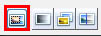 in the toolbar to open a portal view. The portal viewer will open and you will see the Landsat image in the Portal window and the MODIS image behind. The Portal tool uses the first non-portal layer in the Layer Manager as the display layer, and the second layer as the source in the Portal window. Use the cursor to drag the portal view around, you can change the size of the portal window by dragging the corners to re-size. You can open up multiple portal views at a time to display different layers.
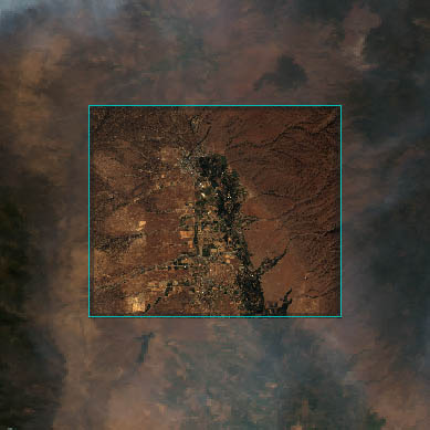
 Example of fire perimeter ROIs for a different fire