Lab 12: Lidar in ArcGIS

Introduction

In this lab we will work with a lidar data set ArcGIS Pro. The lidar point cloud data is typically stored as a LAS file (.las). A LAS file is an industry-standard format for storing X, Y, and Z point data (lidar). We will looks at different ways to visualize the lidar data in both 2D and in 3D using ArcGIS Pro. In this lab we will also learn how to create lidar derived raster datasets. In this lab we will use the Lidar data to create high resolution a digital elevation model (DEM), digital surface model (DSM) and finally a canopy height model (CHM).

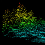
About the Data: The lidar point cloud data for this lab was acquired through the USGS 3D Elevation Program (3DEP). The point cloud data is available for download in a compressed LAZ file (.laz) format through the USGS National Map Download site. This data encompasses the 599-acre recently created McKinleyville Community Forest. The McKinleyville Community Forest consists of second-and third growth Sitka spruce, redwood and Douglas fir. The lidar data was collected in the fall of 2022.

Learning Outcomes

• Use ArcGIS Pro to visualize lidar data in 2 and 3 dimensions.
• Create Digital Surface Models from lidar point data.
• Create Digital Surface Models for lidar point data.
• Create canopy height models from DEM and DSM
• Visualize data in 3D using Arc GISPro.

Set up your Workspace

First we need to set up our workspace.

1. Locate the Desktop and create a new folder named Lab_12. Create two subfolders, one name Originals and one named Final.
2. Download the Lab 12 data zip file and extract the data into the Originals folder. The lab data folder includes a shapefile with the forest boundary and separate folders with the LAZ files (lidar point cloud files). Each point cloud file (or tile) covers approximately 0.5 mile x 0.5 mile square or around 150 acres. LAZ is the compressed format of the standard LAS files, the LAZ files will be decompressed using ArcGIS Pro in next steps.

Creating and Viewing LAS Datasets

3. Start ArcGIS Pro and create a new project in your Lab 12 Final folder. In the Catalog Pane, add a folder connection to your Lab 12 folder then make a new folder named LAS_Files in the Originals folder .
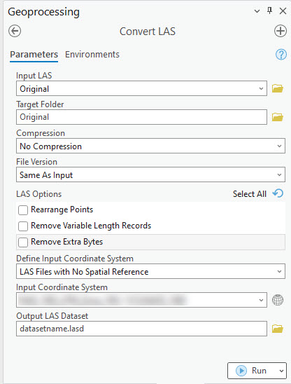
4. The LAZ (.laz) files need to be extracted to the LAS (.las) format before they can be loaded in ArcGIS Pro. From the Geoprocessing pane search for or navigate to the Convert LAS tool and open the tool.
5. The Convert LAS tool can convert single files or entire folders. Select the folder containing the LAZ files as the Input LAS. This will convert all LAZ files (.LAZ) located in this folder. Select the LAS_Files folder as the Target Folder. This will place the extracted LAS files into the this folder when the process is complete. Compression should be set to No Compression (this extracts or decompresses files) and leave all of the LAS Options unchecked and LAS Dataset field blank. Click Run to convert the files.
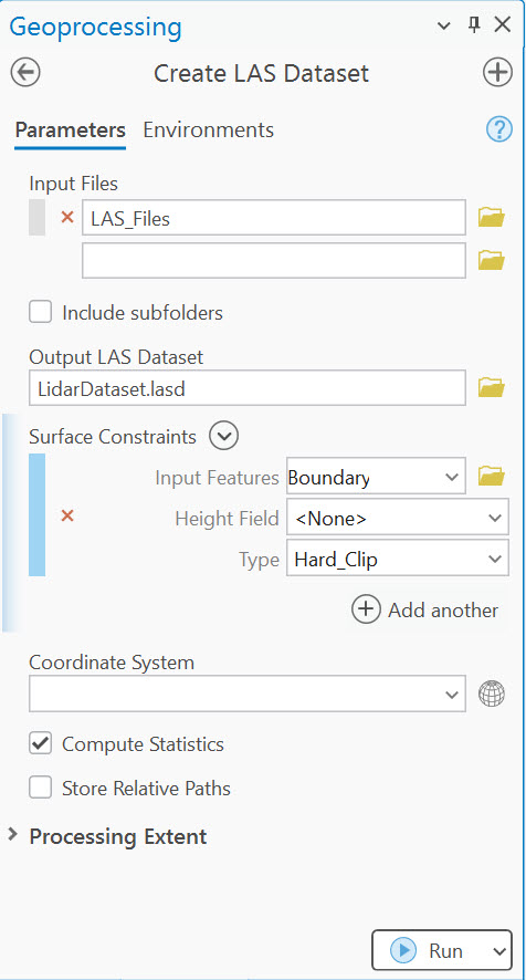
6. Nothing will appear after the tool runs, but the LAZ files should have been extracted in the LAS_Files folder. Check in the Catalog pane to make sure the LAS files are in the approriate folder. We now need to create an LAS Dataset to manage and display of the LAS files. Search for and open the Create LAS Dataset tool from the Geoprocessing pane.

What's a LAS Dataset

A LAS dataset stores references to one or more LAS files, as well as to additional surface features. The LAS dataset allows you to examine .las files in their native format quickly and easily, providing detailed statistics and area coverage of the lidar data contained in all of the .las files. The LAS dataset does not import point data contained in the LAS format file, but only stores a reference to those files. The LAS Dataset allows you to quickly view statistics and information for all the lidar points clouds within a study area. LAS Datasets also aid in creating surfaces rasters such as digital elevation models (DEMs) and other digital surface models.

7. In the Create LAS Dataset tool, select the LAS_File folder as the Input File, this will add all of the LAS files in the folder to the datatset. Set the Output LAS Dataset to save as LidarDataset in your Originals folder. Under Surface Constraints add the Community Forest Boundary shapefile as the Input Feature and set the Type to Hard_Clip. Click Run to create the LAS Dataset.
   

   What's a Surface Constraint?
   
   Surface constraints are breaklines, water polygons, area boundaries, or any other type of surface feature enforced in the LAS dataset. Surface constraints are feature classes or shapefiles. Surface constraints are enforced when the LAS dataset is drawn as a triangulated irregular network (TIN) surface model and when geoprocessing tools are run. For example, when a Digital Elevation model is generated from the point cloud data, only points within the Surface Constraint boundary will be included.

8. After the tool runs, the LAS Dataset should automatically be added to your map. You only will see a series of red squares outlining of the data extent. This is normal, by default not all of the points are displayed because there are too many. If you zoom in you should be able to see the data. You will need to zoom in significantly for the points to appear (scale of ~1:1000).
9. In the Catalog pane, right-click on the LAS Dataset you created in the previous step (.lasd) and select Properties. This will bring up the LAS Dataset properties and statistics.. In the different Dataset properties you will find the total number of LAS points in all of the files, statistics for the individual LAS files and summaries of the returns, classifications and other data attributes. Now is a good time to open the Lab 12 Worksheet in Canvas. Note that you will not find the LAS statistics if you right click on the file in the Contents pane, you must access the properties from the Catalog view to see the full statistics and properties.
10. Click on the Statistics option and if needed click the Calculate button to produce the statistics for this LAS dataset from the LAS files you added.
    Now you will see information about the LAS files, including the point counts, classifications and returns. The LAS Files tab includes information about the linear point spacing for each of the LAS files while the Statistics includes information about the classification and attributes. Note that you can highlight and copy/paste the LAS file statistics into a spreadsheet to view the information.  Make sure the Horizontal and Vertical Coordinate System are specified note the units. Close the LAS Dataset properties when you are done. You will need some of this information to questions on the lab worksheet. 
11. Return to your map and zoom back into the LAS data until you can see points. Now we can check out different ways to visualize the data points in 2D. Click on the .lasd file in the contents pane to select it as the active layer. Now there will be a LAS Dataset Layer tab in the main ribbon. Click the LAS Dataset Layer tab. This controls how the LAS is displayed.
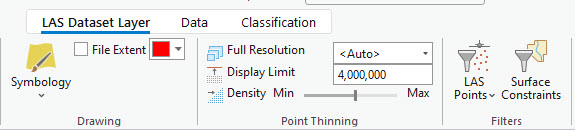
12. First change the Point Thinning options. This allows some control over how many points can be rendered on the map. The density allows for more or less points. The maximum Display Limits is 100,000,000. Try increasing the display limits (if your computer is having a hard time rendering the points you may want to reduce the limit and density) and changing the Density.
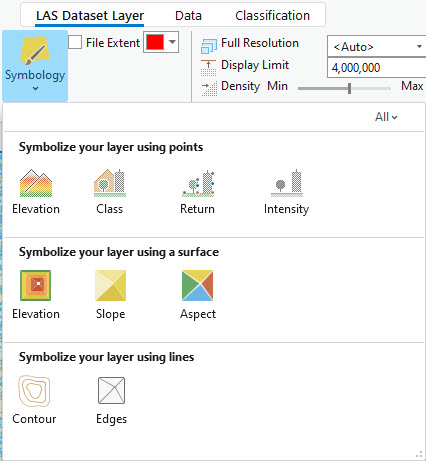
13. Check out the Symbology options by clicking the arrow below the Symbology icon. You can visualize the points by different attributes, including Elevation, Class and other attributes (varies depending on the data). You can also symbolize the layer as a surface rather than points. Try out all of the different symbology options. When you are done exploring the different visualization option, return you Symbology to visualiza the layers as Points based on Elevation.
14. The Filters group on the LAS Dataset Layer tab set allows you to change the display of the data and display selected classes or returns. Once the filter options have been chosen, any further analysis or symbology changes will honor the selected filters. This means any statistics run or files created will be created using only the filtered points. Make sure the LAS Dataset is selected before trying to change the filters. Try different combinations of filters and symbology options. Reset the filters to All Points when you are done exploring and the symbology to Points.

View LAS Data in 3D

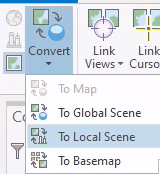
15. Any 2D map can be converted to a 3D scene for data visualization, exploration, or analysis. Click View from the main ribbon and select Convert >To Local Scene. This will convert the current map to a 3D enabled scene.
16. Check out the LASD layer in 3D. In the 3D view you can see all points and pan/move the area around using the Explore tool (under the Map tool ribbon), see more: 3D Navigation in ArcGIS Pro. Explorer the scene by zooming in and panning around
17. You can control the display of the LAS points in the 3D map the same as you can in 2D. Play around with the LAS data filters and symbology options. When you are done return to the 2D map, we will return to the 3D scene later.

Creating a Digital Surface Models from LAS Datasets

First we will create a Digital Elevation Model (DEM) from the Ground Returns. A Digital Elevation Model (DEM) is a representation of the bare ground (bare earth) topographic surface of the Earth excluding trees, buildings, and any other surface objects. To create a DEM we will filter the points to only include data points that are classified as ground or water.  

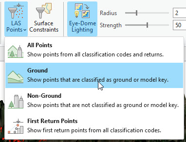
18. In the 2D Map, filter the LAS dataset so only ground points are displayed. This will ensure only ground points are processed when we create our DEM in the next step.
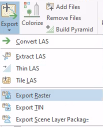
19. Now we will use the LAS Dataset to Raster tool to generate different digital surface models starting with a bare earth DEM. Either select the LAS Dataset to Raster tool from the geoprocessing menu or go to the Data tab under the main ribbon and select Export → Export to Raster.
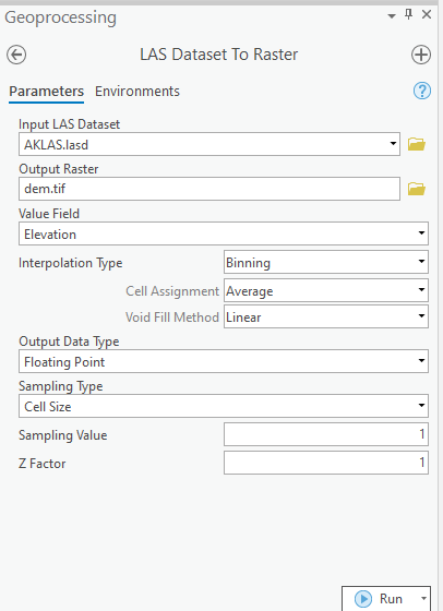
20. Under Input LAS Dataset, select the LAS Dataset (.lasd). Make sure you select this from the drop-down not by clicking on the file folder, this will preserve the filter we set in the previous steps.  Save the output raster as "DEM.tif” in your Final folder.  Keep the Value Field as “Elevation” as we want to create an elevation raster.  
21. Under Interpolation Type keep “Binning” selected and under Cell Assignment Type select “Average”.  The last thing we are going to change is the Sampling Value, set this to “1”.  This defines the spatial resolution of our output raster, which will be 1 meter (the unit of the sampling value is determined by the horizontal coordinate system). 
22. The Digital Elevation Model (DEM) should now be in your viewer. This is a "bare earth" model that represents the elevation of the terrain without any vegetation. Make note of the minimum and maximum values of the DEM, these represent the highest and lowest areas of terrain (ground) in the image.

Creating Digital Surface Model of the First Returns (Canopy)

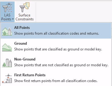
23. Right click on the LASD layer in the Table of Contents and select Properties. In the LAS Filter tab this time, check 1 under Returns and make sure all of the classes are selected. If there are classes labeled as Noise or High Noise these should be unchecked and left out of the analysis. Note that not all LAS datasets have Noise classifications. This filters the points so only the first returns will be shown, the first returns represent the highest point in the area. You can also filter to first return by using the drop-down on the LAS Points option on the main toolbar.

24. We will now follow a similar process that we used to create the DEM but this time we will be creating a digital surface model raster of the first returns (canopy). Either select the LAS Dataset to Raster tool from the geoprocessing menu or go to the Data tab under the main ribbon and select Export Export to Raster.
25. Keep the Value Field as “Elevation” as we still want to create an elevation raster. Under Interpolation Type keep “Binning” selected and under Cell Assignment Type select “Maximum”, this will use the maximum point elevation. The last thing we are going to change is the Sampling Value, set this to “1” to define the spatial resolution of our output raster (1 m in this case). Save the output raster as “DSM.tif” in your folder. Press “OK”. Now the DSM file should have automatically been added to your viewer.

Creating a Canopy Height Model (CHM)

With both the DEM and DSM generated from the lidar data it is possible to estimate the canopy height above the ground. The DSM is essentially the height of the canopy above sea level. We want to create a raster that solely represents the height of canopy above ground. This can be done by simply subtracting the DEM from the DSM, which produces a canopy height model (CHM).

26. Using the Spatial Analyst Math tools we will create a canopy height raster by subtracting the two rasters.  Find the Minus tool in the Geoprocessing pane (Spatial Analysis Tools→ Math → Minus).
27. For Input Raster 1 select the canopy surface model "DSM.tif" and for Input Raster 2 select the DEM "DEM.tif", so DSM-DEM = CHM (Canopy Height Model).  Save the output raster in your Final folder as “CHM.tif” and click OK.
28. You will now see the canopy height raster in your viewer.  The values in this raster represent the height of the vegetation above ground (in meters in this example).  You may want to change the symbology to a different color ramp that better displays the data. Make note of the maximum value of the CHM.
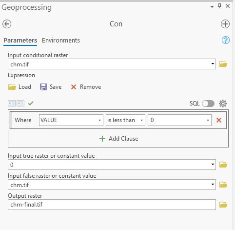
29. Depending on the data, you may encounter negative CHM values, these values are due to noise that may not have been properly filtered out the data (like birds or other features). We will remove any negative values (noise) using the Con geoprocessing tool to recalculate any negative values to a value of zero. In the geoprocessing pan select the Con tool by searching for it or by locating it under Spatial Analysis Tools→ Conditional → Con.
30. In the Con tool window, select the CHM files has the Input conditional raster. In the Expression box enter Value < 0, this will apply the tool only to pixels where the canopy height value is less than 0. Type "0" in the Input true raster or constant value. This will replace any values less than 0 (negative values) with 0. In the next box, Input false raster or constant value select the CHM file. This will use the existing CHM values for all areas where the values are greater or equal to 0. Save the file as CHM-final.tif in the Finals folder and hit OK.


 

31. You now have a cleaned-up, final Canopy Height Model (CHM). The pixel values in this CHM represent the maximum above ground canopy height in the pixel. Now let's look at the details of the canopy height layer. in the Contents pane, right-click, select "Properties", go to the "Source" tab, and then find the "Statistics" section. This will show minimum, maximum and mean canopy height values for the data.
32. Repeat the above step for the Digital Elevation Model (DEM). Note the min/max/mean values.
33. Now we will view a histogram of the canopy height data (CHM) With the CHM layer selected, under the Raster Data tab go to Create Chart > Histogram. The Histogram tool appears or right click on the layer and select Create Chart > Histogram.
34. In the Chart Properties pane, select "Band_1" as the Number variable. This is the band with the canopy height data. Look at the histogram, it shows the distribution of values and how many pixel in the image have that value range. Review the max values and see how many (if any) pixels have these values. Use the histogram to help answer the questions in the Lab 12 Worksheet.
35. You also have all the information needed to complete the Lab 12: Worksheet in Canvas. You may need to revisit steps 8-10 to view the LAS Dataset properties and Statistics in Catalog to complete the worksheet.

Creating Hillshades with Raster Functions

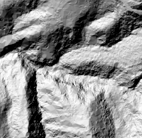
Raster functions are operations that apply processing directly to the pixels of imagery and raster datasets, as opposed to geoprocessing tools, which write out a new raster to disk. Calculations are applied to the pixels of the original data as the raster is displayed, so only pixels that are visible on your screen are processed. These tools are a great way to quickly preview an operation or to create layers for visualization. If you need to save the file or use it in future analyses the geoprocessing tools are more appropriate. Hillshades are rasters that appears to be a photo from above the sea, shaded by the sun. They rarely used for analysis but are one of the most common backgrounds used with maps. You can make a simple hillshade very quickly with just a DEM file. Hillshades are also useful base layers to use when layering imagery over a surface.

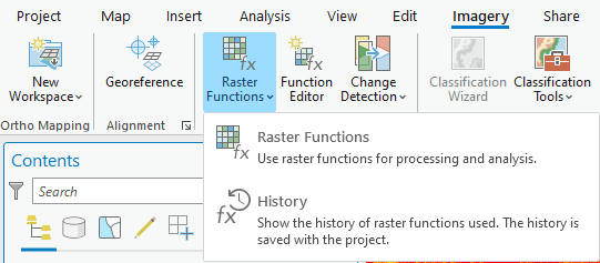
36. Under the Imagery Tab navigate to the Raster Functions button and click on the Raster Functions. This will launch the Raster Functions pane on the side. There are many different functions to choose from.
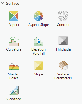
37. Navigate to the Surface functions in the Raster Functions tool pane. Select the Hillshade option.
38. Create a hillshade using the DEM as the input file (you can keep all of the default settings).
39. Repeat the above process an create two more hillshades, one for the CHM and one for the DSM, you should have three hillshades when you are done.

Arranging Data and Creating Maps

40. First we will create layer groups to organize out layers. Right click on Map in the Contents and select New Group Layer.  Click on the name and rename it to “Elevation”.  Repeat this again and create a second group, and rename the second layer group as “Canopy”. Drag the layers so the final CHM and CHM & DSM hillshades are under the Canopy group layer an the DEM and DEM hillshade under the elevation group. This will allow you to turn on and off all layer in the group with one click and makes organizing data easier.
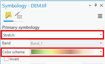
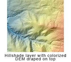
41. Let’s update the symbology for the DEM. Select the DEM file and go the Symbology and change the Stretched symbology to color ramp instead of the default grayscale ramp. The colors correspond to the different elevations.
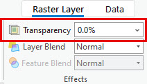
42. In order to display the elevation data as a layer on top of the hillshade we will need to set the transparency of the elevation layer. Under the Appearance option change the transparency to 50% for the DEM.   This will set the transparency to 50% for this layer allowing the hillshade layer to show through, note that the DEM layer should be on top of the hillshade. 
43. Repeat this same process for the Canopy Height (CHM) layer, choose different color symbology for the DEM and CHM. Keep the default grayscale symbology for the Hillshade layers.
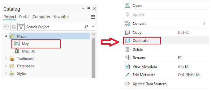
44. Remove the default esri basemaps from the map and save your project. In the Catalog pane, create a duplicate of your existing map by right-clicking on the map and selecting Duplicate. Re-name your two maps, so one is named Elevation and the other Canopy. Open both of the maps (one should already be open), now you have a seperate map for Elevation and Canopy.
45. Create a map layout or two separate map layouts, (your choice) that shows the Elevation (map 1) and Canopy Height (map 2) of the forest. Each map should include the surface model (DEM or CHM) and applicable hillshade and should also include titles, legend, north arrow, scale bar and data sources/map author. The maps can be any size or layout style. Tips and Trick for Working with Legends in ArcGIS Pro
46. Export map (or maps) in PDF or JPG format at 300 dpi resolution.

Create a 3D View and Map

47. Return to the 3D map and add your elevation (DEM) and canopy height rasters (CHM). Uncheck or remove the LAS Dataset layer to make the 3D map render more quickly.
48. Right-click on the Ground element under the Elevation Surfaces group at the bottom of the Content Pane and select Add Elevation Source. Select the DEM.tif and DSM.tif rasters from the project folder then click OK. Remove the default "WorldElevation3D/Terrain3D" layer.
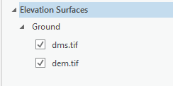
49. Any layer added to the 2D layers group will now be draped over the elevation surface. You should see Note that the DEM is the bare ground elevation and terrain, while the DSM includes the elevation of the above ground vegetation in addition to the ground. Turn the two elevation surface layers on and off to see the differences between the two.
50. Now add a Satellite Imagery 2D Basemap to your 3D map. This will display a recent satellite image or the area. Try turning on and off the different layers and experimenting with the display options. Pick a layer (DEM/CHM/satellite imagery) to display in your final 3D map, either the imagery, the elevation or the canopy height.
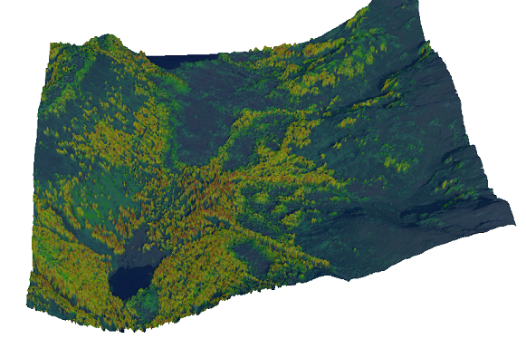
51. The last step is to create a simple map layout with our 3D image. Create a new layout and select the 3D map as the Map Frame. Zoom out and rotate the map so the 3D nature is apparent. Add a title and north arrow to your map. Export your image by going to Share → Export Map. Save your image in your Lab 12 folder as a JPG.

Complete the Lab 12: Worksheet in Canvas

Lidar Derived Maps and Images (Upload to Canvas)

Upload the following to Canvas. Note: the first two can be combined into one map with side-by-side data frames if desired.

• Map that shows the Elevation with shaded relief. Include title, legend, north arrow and scale (PDF/JPG).
• Map that shows the Canopy Height (CHM)with either the CHM or DSM shaded relief. Include title, legend, north arrow and scale (PDF/JPG).
• Exported 3D map image with imagery/elevation/canopy height (your choice) draped over 3-D surface model.