 R for Spatial Statistics
 Generalized Additive Models (GAMs)
Creating a GAM Model
GAMs are an extremely powerful method for spatial modeling. GAMs add "smoothing" functions to the predictors to provide great flexibility in the nature of the response to the predictors.
Before starting below, you'll want to have a dataset that contains sampled values with associated predictor values. You'll also want to have a similar dataset setup with points covering the entire sample area and the predictor values in columns. Things will go easier if you have the names of the predictor values in both files matching exactly.
R makes creating GAMs extremely easy. The syntax is very similar to lm() with only a few additional parameters. To get started, you'll want to load the "mgcv" library and a data set into a data frame an use remove any null values.
require(mgcv) # load the GAMs library

# Read the data
TheData = read.csv("C:/ProjectsModeling/Cali_5Minute/DougFir_CA_Predict 4.csv")

# Remove any NA (null) values
TheData=na.omit(TheData)
To run a GAM, you provide a response variable and a series of predictor variables just as you did with a linear model. The difference is that you'll want to pass each predictor variable into an "s()" function for "spline". These functions will provide a smoothed spline curve. You'll also want to provide a distribution function for the response variable and a "link" function to link the response variable into the linear portion of the model. Typical functions are:
| Type of data | Family of Distributions | Link Function |
|---|---|---|
| Continuous data | gaussian | identity |
| Binary data (true/false) | binomial | logit |
| 0-based continuous | Gamma | inverse |
| Counts | poisson | log |
The default family is "gaussian" and the format to specify the distribution is:
TheModel = gam(Height~s(AnnualPrecip),data=TheData,family=gaussian())
TheModel = gam(Height~s(AnnualPrecip),data=TheData,family=binomial())
TheModel = gam(Height~s(AnnualPrecip),data=TheData,family=Gamma())
TheModel = gam(Height~s(AnnualPrecip),data=TheData,family=poisson())
The last parameter that you will want to provide is a "gamma" parameter which specifies the amount of smoothing to apply to the spline curves. This can be interpreted as the number of "knots" used for the spline curves for each predictor variable. Below is an example.
To use the "predict.gam()" function to predict values from our model we will need to "attach()" the data set so the names of the columns can be matched between to the data set for the prediction.
Warning: after using a variable with "attach()" remember to detach it with "detach()". If you don't, the number of attached variables will continue to increase causing confusion and lots of warning messages. Also note that "detach()" requires that the variable name be in quotes. You can check the values that are attached with the function "search()".
# We have to use "attach()" because predicting values later on requires it
attach(TheData)

# the family is gaussian by default but the gamma should be changed from 1 to smooth
TheModel=gam(Height~s(AnnualPrecip),data=TheData,gamma=1.4) # Recommended smoothing factor

# remember to "detach()" the variable after using it
detach("TheData") # note the quotes
"summary()" provides similar values to a GLM except that we'll need to run the "AIC()" function to see the AIC value.
# The summary does not provide an AIC but "AIC()" does
summary(TheModel)
AIC(TheModel)
You can also get the likelihood for a GAM with:
logLik.gam(TheModel)
You can find the number of knots (esimated parameters) for each independent variable by using the code below (courtesy of Katelyn Brady).
# Extract information about the smooth terms
smooth_terms <- TheModel_8$smooth
# Print number of knots for each smooth term
for (smooth_term in smooth_terms)
{
	cat("Smooth term:", smooth_term$term, "\n")
	cat("Number of knots:", smooth_term$bs.dim, "\n\n")
}
The plots below are referred to as "partial dependence plots" because they only show the dependence between the predictor and response variables for one predictor. The standard "plot()" function will show the plots but you can also specify "pages=1" to have them all appear on one page.
# Plot the model, including confidence intervals
plot(TheModel)

# All the plots on one page
plot(TheModel, pages=1, scale=F, shade=T)
Below is an example output from a rather weak model (you can do better). The gray areas around the response curves are the confidence intervals. The "grass" at the bottom of the graphs shows the number of samples at each predictor values. The confidence intervals are very large on the left because the number of samples is also very low.
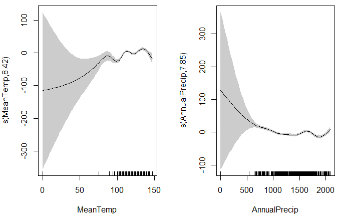
GAM Plots
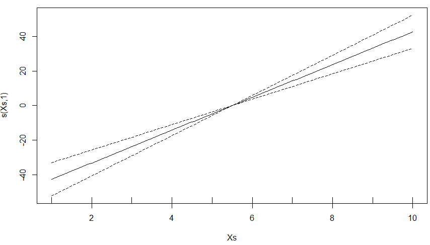
When a GAM does not have enough data to create a spline curve, it will create a linear model. The performance statistics for this model should be accurate but the confidence interval for the model will not be. Below is an example.
Creating a Predicted Spatial Surface
By default, the function "predict.gam()" will add predicted values to your existing dataset. You can also provide a different dataset with predictor values that include the entire sample area. If the headings for the files match the original file then the code below will produce new, predicted values. This is how you can create a model from a set of points and then predict for a different area such as a grid.
# read in the data with the same covariates over the entire study area
# note that the covariates must have exactly the same names as were used
# to create the model
NewData = read.csv("C:\\Users\\jim\\Desktop\\GSP 570\\DougFirGAM\\DougFir_AllCA_Covariates.csv")
# create the prediction
Prediction=predict.gam(TheModel,NewData,type='response')

# Create a new data table that includes the NewData and the prediction
FinalData=data.frame(NewData,Prediction)

# Plot the prediction against the covariate
plot(FinalData$AnnualPrecip,FinalData$Prediction)

# Save the prediction to a new file
write.csv(FinalData, "C:/ProjectsModeling/ModelOutput.csv")
Now you can convert the prediction into a new layer in a GIS package. Remember to use the original extent and pixel size for the raster.
Plotting the original data and the prediction
You can combine the original data and the prediced points from the model into a single chart.
plot(TheData$AnnTemp,TheData$PopCount) # plot the data
points(TheData$AnnTemp,ThePrediction,col=2,pch="o") # plot the prediction
Extra credit for the first person to figure out how to plot the original points with the model and a confidence interval.
Vewing the GAMs with the correct Y-Axis
You've probably noticed that the Y-Axis with GAMs is not what you would expect. This is because the plots only show the contribution to the model for one predictor at a time. This does not include the Y-Intercept value. You can see this by fitting the original data to the model with the "fitted()" function.
plot(TheData$MaxTemp,fitted(TheModel))
Plotting GAMs in 3D
You can also plot GAMs in 3D using the rgl library.
require(rgl)

plot3d(TheModel)
Additional Resources
R Package: Generalized Additive Models with Integrated Smoothness Estimation
Excellent Book on linear modeling: Generalized Additive Models: an introduction with R
How to solve common problems with GAMs
Slide Presentation: Introduction to Generalized Linear Models
An introduction to mgcViz: visual tools for GAMs - examples of creating very nice graphics for GAMs.
GAM: The Predictive Modeling Silver Bullet - Details on how to fit maps