 R for Spatial Statistics
 Linear Regression
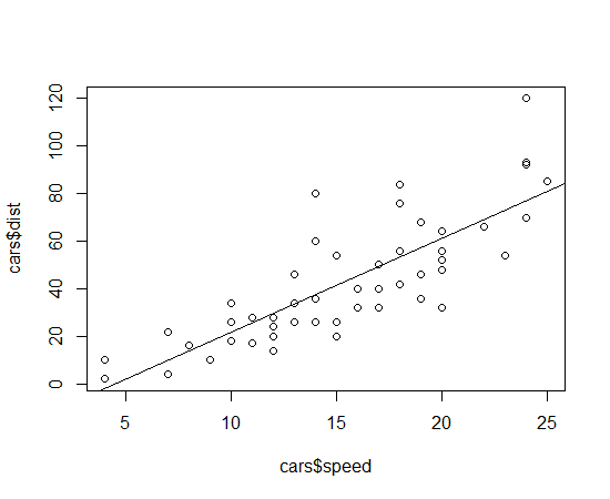
To get started, we'll load the "stats" library which contains a number of example data sets including a small table of speeds and distances for cars. Enter the code below to make sure the "stats" library is loaded and then plot speed against distance.
require(stats)
plot(cars$speed,cars$dist)
You can display data by just typing the name of the variable. You can also check the length of a vector or matrix with the "length()" function.
length(cars$speed)
To create a linear model, you can use the "lm()" function. The code below specifies the column "dist" within the "cars" table and the column "speed". The tilde character (~) indicates that we want to regress speed as the predictor (independent) variable against distance as the response (dependent) variable. Note that the order is opposite of the "plot()" command.
RegressionModel=lm(cars$dist~cars$speed)
We can then add the regression model as a straight line with "a" and "b" parameters with the "abline()" function.
abline(RegressionModel)
Your plot should now appear similar to the one below.
You can print out the coefficients for the model by just entering the name of the model:
> RegressionModel

Call:
lm(formula = cars$dist ~ cars$speed)

Coefficients:
(Intercept)   cars$speed
    -17.579        3.932
The output above shows the original call that was made and the intercept and slope of the line for th linear regression. The image below shows how the coefficients in R relate to the coefficients in a multiple linear equation.

There is more information available if you use the summary() function. Take some time reviewing the values below with the definitions that follow as this is a typical output from a regression function in R and you'll be seeing a lot of them.
Call:
       lm(formula = cars$dist ~ cars$speed)

Residuals:
       Min      1Q  Median      3Q     Max
       -29.069  -9.525  -2.272   9.215  43.201


Coefficients:
       Estimate Std. Error t value Pr(>|t|)
       (Intercept) -17.5791     6.7584  -2.601   0.0123 *
       cars$speed    3.9324     0.4155   9.464 1.49e-12 ***
       ---
       Signif. codes:  0 '***' 0.001 '**' 0.01 '*' 0.05 '.' 0.1 ' ' 1

Residual standard error: 15.38 on 48 degrees of freedom
       Multiple R-squared:  0.6511,	Adjusted R-squared:  0.6438
       F-statistic: 89.57 on 1 and 48 DF,  p-value: 1.49e-12
Call: Original function that was executed
Residuals: The min/max and quantiles for the distribution of the residuals, we would expect the "Median" to be near 0
Coefficients: The coefficients of the fitted function and how significant they are.
- Estimate: Value of the coefficient
- Std. Error: Standard error
- t-value: Indicates if this value is meaningful in the model
- Pr(>|t|): p-value, the smaller the value the better. The stars to the right indicate how "good" the p-value is.
- "Signif. codes: this is just a legend for the number of stars next to the p-values
Residual standard error: standard deviation of the residuals. For a normal distribution, the 1st and 3rd quantiles should be 1.5 +/- the std error.
- Degrees of Freedom: Number of observations minus the number of coefficients (including intercepts). The larger this number is the better and if it's close to 0, your model is seriously over fit.
- Multiple R-squared: Indicates the proportion of the variance in the model that was explained by the model. Perfect is 1, none is 0.
- Adjusted R-squared: Attempts to adjust for R-squared increasing as the number of explanatory variables increases.
F-statistic: A test to see if a model with fewer parameters will be better
- p-value: a low value indicates that our model is probably better than a model with fewer parameters (i.e. there is little chance that the results are random)
Warning: Remember that "explaining" variance is an indication of correlation and not necessarily causation.
Plotting The Model Residuals
Now, run the model plots to produce four graphs that can be used to interpret the model:
plot(TheModel)
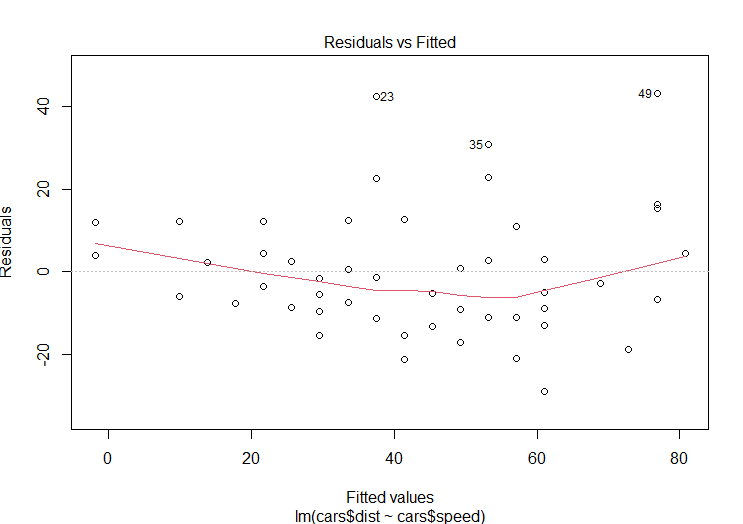
The "residuals vs. fitted" plot shows the residuals on the y-axis and the fitted values (y values from the samples) on the x-axis. Another way to think of this is that the x-axis shows the independent value along the trend line and the y-axis shows the difference between this value and the sample value (i.e. the residual).
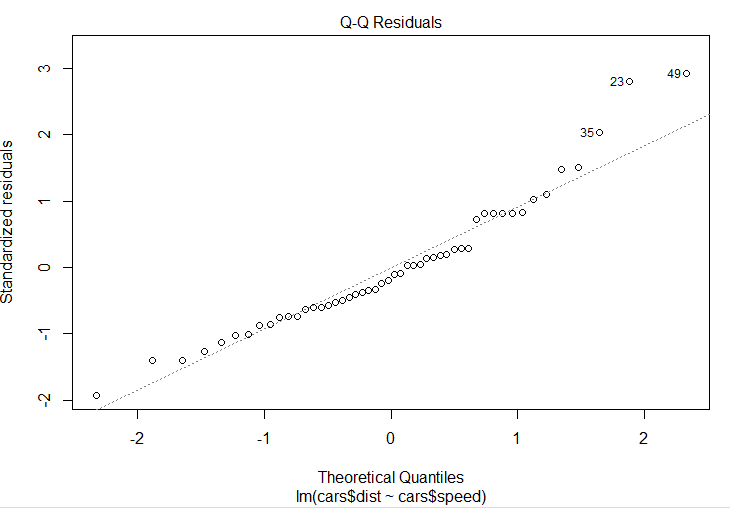
The next graph shows a Normal Q-Q plot. This plot breaks the original data into "quantiles" or buckets where each bucket as about the same number of data points. Then the mean value of each bucket is plotted for the original data against what we would expect from the model. The dashed line shows the expected value.
I'm not sure about the next two charts - let me know if you find a use for them!
Additional Resources
Easy to read explanation of lm in R